淘宝用户行为分析
漏斗模型是一种常用的用户行为分析工具,主要用于分析用户在不同阶段的转化率。在电商领域,漏斗模型通常用于分析用户从浏览商品到最终购买的各个阶段的转化情况。点击(Click)添加购物车(Add to Cart)购买(Purchase)通过漏斗模型,可以识别用户在哪个阶段流失最多,从而采取相应的优化措施。
数据分析模型
数据来源自阿里云天池的阿里移动推荐算法竞赛,以淘宝app平台在2014年11月18日-12月18日的数据为数据集。
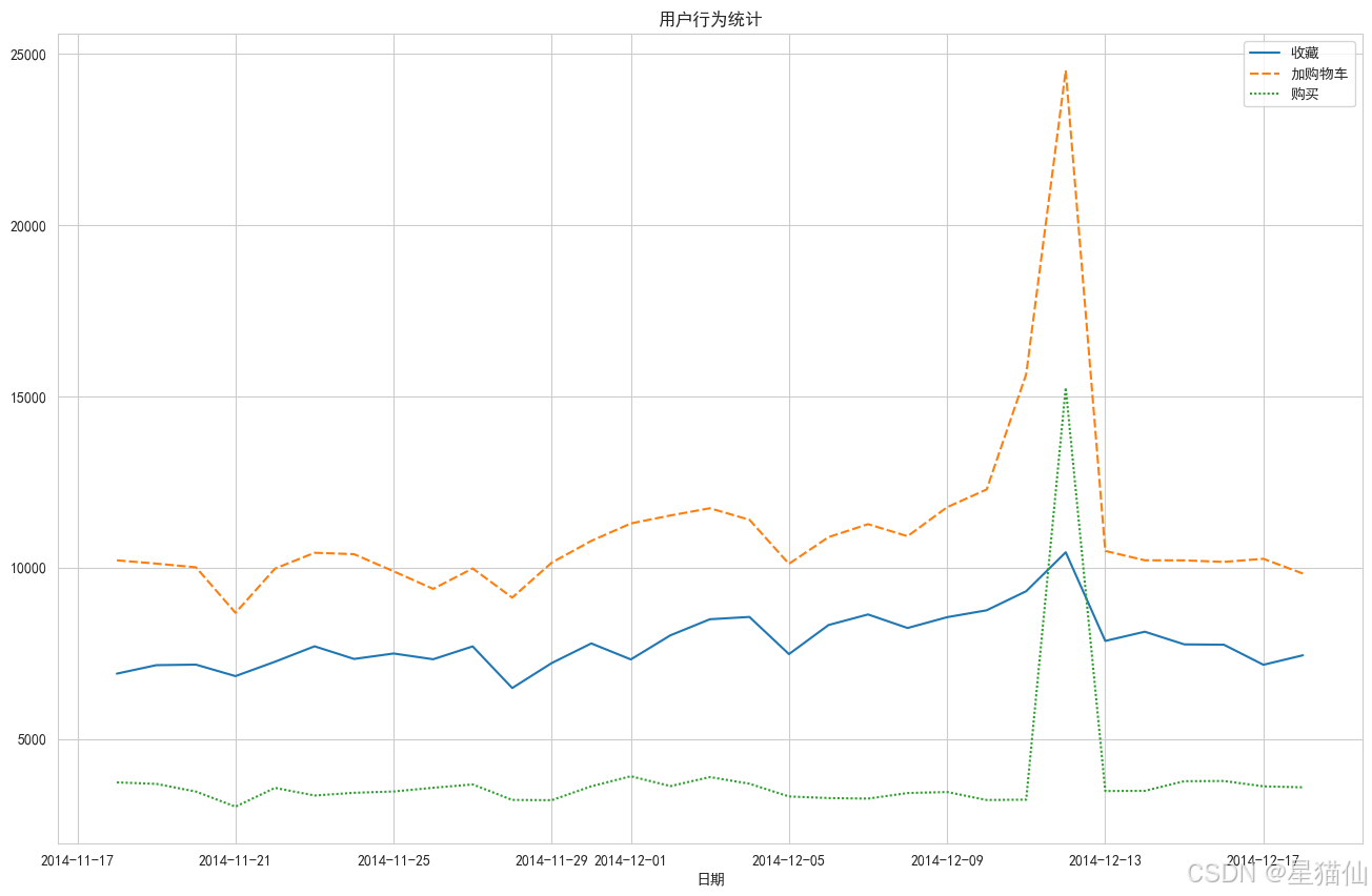
值得注意的是,“双十二”大型促销活动的数据也会大量包含在数据集中,初步推断“双十二”当天的数据应该会出现井喷现象。
数据包含4个字段,分别是
user_id: 用户id
item_id:商品id
behavior_type:用户行为,1:点击,2:收藏,3:添加购物车,4:购买
user_geohash: 用户地理位置hash值
item_category:商品类别
time:时间戳
在这里通过行业的指标对淘宝用户行为进行分析。结合常见的电商数据分析模型与python数据分析及可视化,进行分析任务:
1、每日pv统计、每日uv统计;
2、每日用户行为趋势;
3、漏斗模型:用户行为转化分析;
4、周期内用户行为频率。
1.数据读取
parse_dates: 这个参数用于指定哪些列应该被解析为日期时间类型。在这个例子中,['date']表示将date列解析为日期时间格式。infer_datetime_format: 当设置为True时,pandas 会尝试推断日期时间格式,从而加快解析速度。这对于包含大量日期时间数据的列特别有用,可以提高读取效率。
import pandas as pd, numpy as np, matplotlib.pyplot as plt, seaborn as sns

#提前指定好数据类型,以降低内存占用
columns_types = {'user_id':'int32', 'item_id':'int32', 'behavior_type':'category', 'item_category':'int16'}

df = pd.read_csv('./阶段2--Python数据分析实战/tianchi_mobile_recommend_train_user.csv',
                 dtype=columns_types, parse_dates=['time'],infer_datetime_format=True)

print(df.info(memory_usage='deep'))
C:\Users\Lenovo\AppData\Local\Temp\ipykernel_33996\922392374.py:6: FutureWarning: The argument 'infer_datetime_format' is deprecated and will be removed in a future version. A strict version of it is now the default, see https://pandas.pydata.org/pdeps/0004-consistent-to-datetime-parsing.html. You can safely remove this argument.
  df = pd.read_csv('./阶段2--Python数据分析实战/tianchi_mobile_recommend_train_user.csv',


<class 'pandas.core.frame.DataFrame'>
RangeIndex: 12256906 entries, 0 to 12256905
Data columns (total 6 columns):
 #   Column         Dtype
---  ------         -----
 0   user_id        int32
 1   item_id        int32
 2   behavior_type  category
 3   user_geohash   object
 4   item_category  int16
 5   time           datetime64[ns]
dtypes: category(1), datetime64[ns](1), int16(1), int32(2), object(1)
memory usage: 715.8 MB
None
df.head()
| user_id | item_id | behavior_type | user_geohash | item_category | time | |
|---|---|---|---|---|---|---|
| 0 | 98047837 | 232431562 | 1 | NaN | 4245 | 2014-12-06 02:00:00 |
| 1 | 97726136 | 383583590 | 1 | NaN | 5894 | 2014-12-09 20:00:00 |
| 2 | 98607707 | 64749712 | 1 | NaN | 2883 | 2014-12-18 11:00:00 |
| 3 | 98662432 | 320593836 | 1 | 96nn52n | 6562 | 2014-12-06 10:00:00 |
| 4 | 98145908 | 290208520 | 1 | NaN | 13926 | 2014-12-16 21:00:00 |
df.info()
<class 'pandas.core.frame.DataFrame'>
RangeIndex: 12256906 entries, 0 to 12256905
Data columns (total 6 columns):
 #   Column         Dtype
---  ------         -----
 0   user_id        int32
 1   item_id        int32
 2   behavior_type  category
 3   user_geohash   object
 4   item_category  int16
 5   time           datetime64[ns]
dtypes: category(1), datetime64[ns](1), int16(1), int32(2), object(1)
memory usage: 315.6+ MB
2.数据预处理
#将字段中的空格去掉,但是这里打印查看,显示没有空格
df.columns
Index(['user_id', 'item_id', 'behavior_type', 'user_geohash', 'item_category',
       'time'],
      dtype='object')
2.1 缺失值处理
# 看看有几个重复值
df.duplicated().sum()
4092866
# 缺失值
df.isnull().sum()
user_id                0
item_id                0
behavior_type          0
user_geohash     8334824
item_category          0
time                   0
dtype: int64
这里发现user_geohash有缺失值,但是缺失值太多,我们先看看缺失值的比例,如果很高就可以删去这个列,如果比例较低,可以尝试用众数来填充,或者用平均值来填充,这里我们先不处理
# 计算缺失值的比例
df.isnull().sum()/df.shape[0]
#还可以这么写:df.isnull().sum()/len(df)
#还可以用apply和lambda函数:df.apply(lambda x:x.isnull().sum()/len(x))
user_id          0.00000
item_id          0.00000
behavior_type    0.00000
user_geohash     0.68001
item_category    0.00000
time             0.00000
dtype: float64
# 删除user_geohash列
df.drop('user_geohash',axis=1,inplace=True)
df.columns
Index(['user_id', 'item_id', 'behavior_type', 'item_category', 'time'], dtype='object')
2.2日期标签的处理
# 因为通过观察发现,time标签的数据特征是时间戳,包含日期和时间,为了方便的去分析每日和同一时间的用户行为,需要把日期和小时分开
df['time'] = pd.to_datetime(df['time'])
df['hour'] = df['time'].dt.hour
df['time'] = df['time'].dt.normalize()#这一步是把时间归一化为当天的零点.
# 如果只是要分割日期与小时,可以用df['time'].dt.date
df.head()
| user_id | item_id | behavior_type | item_category | time | hour | |
|---|---|---|---|---|---|---|
| 0 | 98047837 | 232431562 | 1 | 4245 | 2014-12-06 | 2 |
| 1 | 97726136 | 383583590 | 1 | 5894 | 2014-12-09 | 20 |
| 2 | 98607707 | 64749712 | 1 | 2883 | 2014-12-18 | 11 |
| 3 | 98662432 | 320593836 | 1 | 6562 | 2014-12-06 | 10 |
| 4 | 98145908 | 290208520 | 1 | 13926 | 2014-12-16 | 21 |
下面对处理好的表格标签重命名
df = df.rename(columns={'user_id':'用户名',
                        'item_id':'商品',
                        'behavior_type':'行为',
                        'item_category':'商品类别',
                        'time':'日期',
                        'hour':'小时'})
df.head()
| 用户名 | 商品 | 行为 | 商品类别 | 日期 | 小时 | |
|---|---|---|---|---|---|---|
| 0 | 98047837 | 232431562 | 1 | 4245 | 2014-12-06 | 2 |
| 1 | 97726136 | 383583590 | 1 | 5894 | 2014-12-09 | 20 |
| 2 | 98607707 | 64749712 | 1 | 2883 | 2014-12-18 | 11 |
| 3 | 98662432 | 320593836 | 1 | 6562 | 2014-12-06 | 10 |
| 4 | 98145908 | 290208520 | 1 | 13926 | 2014-12-16 | 21 |
3.数据分析
3.1 PV、UV统计
3.1.1PV统计
PV_daily = df.groupby('日期').count()['用户名'].rename('PV')

pv_daily = data.groupby(data['time'].dt.date).size().reset_index(name='pv')
相同点:
两段代码都计算了每天的访问次数。
最终结果都是一个包含日期和访问次数的 DataFrame。
不同点:
第一段代码假设 ‘日期’ 列已经是以日期格式存储的。
第二段代码从 ‘time’ 列中提取日期部分进行分组,适用于 ‘time’ 列包含时间信息的情况。
第一段代码使用 count() 方法,而第二段代码使用 size() 方法。count() 方法会忽略 NaN 值,而 size() 方法不会。
# PV统计,有两种写法
#写法1
pv = df.groupby('日期')['用户名'].count().reset_index(name = 'PV')
pv.head()

# '''
# 按 '日期' 列进行分组。
# 计算每个分组中 '用户名' 列的计数。
# 将结果重命名为 'PV'。
# '''
| 日期 | PV | |
|---|---|---|
| 0 | 2014-11-18 | 366701 |
| 1 | 2014-11-19 | 358823 |
| 2 | 2014-11-20 | 353429 |
| 3 | 2014-11-21 | 333104 |
| 4 | 2014-11-22 | 361355 |
#写法2
pv = df.groupby('日期').size().reset_index(name='PV')
pv.head()

# '''
# 按 'time' 列的日期部分进行分组。
# 计算每个分组的大小(即每个日期的记录数)。
# 将结果重置索引,并将列名命名为 'pv'。
# '''
| 日期 | PV | |
|---|---|---|
| 0 | 2014-11-18 | 366701 |
| 1 | 2014-11-19 | 358823 |
| 2 | 2014-11-20 | 353429 |
| 3 | 2014-11-21 | 333104 |
| 4 | 2014-11-22 | 361355 |
# 绘图
# 显示中文乱码,需要加上一行处理
plt.rcParams['font.sans-serif'] = ['SimHei']

plt.figure(figsize=(16,6))
sns.lineplot(data=pv, x='日期', y='PV')
plt.title('PV统计')
# plt.xlabel('日期')
# plt.ylabel('PV')
plt.show()

3.1.2 UV统计
UV = df.groupby('日期')['用户名'].nunique().reset_index(name='UV')
UV.head()

# 使用 groupby 方法按 '日期' 列对 DataFrame 进行分组。
# 对每个分组计算 '用户名' 列的唯一值数量,即统计每个日期有多少个不同的用户。
# 将结果重命名为 'UV'。
| 日期 | UV | |
|---|---|---|
| 0 | 2014-11-18 | 6343 |
| 1 | 2014-11-19 | 6420 |
| 2 | 2014-11-20 | 6333 |
| 3 | 2014-11-21 | 6276 |
| 4 | 2014-11-22 | 6187 |
# 绘图
plt.figure(figsize=(16,10))
sns.lineplot(data=UV, x='日期', y='UV')
plt.title('UV统计')
plt.show()

# ---
# 在绘图时,选择使用 `rename` 或 `reset_index` 方式来处理分组后的数据,需要注意以下几点:
#
# ### 使用 `rename` 的注意点
#
# 1. **数据结构**:
# - `rename` 后的结果是一个 Series,而不是 DataFrame。
# - 如果你需要绘制图表,确保所使用的绘图库支持 Series 数据类型。
#
# 2. **索引**:
# - 结果的索引是分组的键(例如日期),这可能会影响某些绘图库的行为。
# - 如果绘图库需要 DataFrame 格式,你可能需要先将 Series 转换为 DataFrame。
#
# 3. **绘图库兼容性**:
# - 一些绘图库(如 Matplotlib、Seaborn)可以直接使用 Series 绘图,但其他库可能需要 DataFrame 格式。
#
# ### 使用 `reset_index` 的注意点
#
# 1. **数据结构**:
# - `reset_index` 后的结果是一个 DataFrame,更适合大多数绘图库。
# - DataFrame 格式通常更灵活,可以更容易地进行多列操作和绘图。
#
# 2. **索引**:
# - 索引被重置为默认整数索引,原来的分组键(例如日期)成为普通列。
# - 这使得数据更容易处理和可视化。
#
# 3. **绘图库兼容性**:
# - 大多数绘图库(如 Matplotlib、Seaborn、Plotly)都支持 DataFrame 格式,可以直接使用 `reset_index` 后的结果进行绘图。
#
# ### 示例代码
#
# #### 使用 `rename` 绘图
#
# ```python
# import pandas as pd
# import matplotlib.pyplot as plt
#
# # 创建示例数据
# data = {
#     '日期': ['2023-10-01', '2023-10-01', '2023-10-02', '2023-10-02'],
#     '用户名': ['user1', 'user2', 'user1', 'user3']
# }
# df = pd.DataFrame(data)
#
# # 计算 UV 并重命名
# UV_daily = df.groupby('日期')['用户名'].nunique().rename('UV')
#
# # 绘图
# UV_daily.plot(kind='bar')
# plt.xlabel('日期')
# plt.ylabel('UV')
# plt.title('每日独立访客数')
# plt.show()
# ```
#
#
# #### 使用 `reset_index` 绘图
#
# ```python
# import pandas as pd
# import matplotlib.pyplot as plt
#
# # 创建示例数据
# data = {
#     '日期': ['2023-10-01', '2023-10-01', '2023-10-02', '2023-10-02'],
#     '用户名': ['user1', 'user2', 'user1', 'user3']
# }
# df = pd.DataFrame(data)
#
# # 计算 UV 并重置索引
# UV_daily = df.groupby('日期')['用户名'].nunique().reset_index(name='UV')
#
# # 绘图
# plt.bar(UV_daily['日期'], UV_daily['UV'])
# plt.xlabel('日期')
# plt.ylabel('UV')
# plt.title('每日独立访客数')
# plt.show()
# ```
#
#
# ### 总结
#
# - **`rename`**:适用于简单的绘图需求,特别是当绘图库支持 Series 数据类型时。
# - **`reset_index`**:适用于更复杂的绘图需求,特别是当需要多列操作或绘图库不支持 Series 数据类型时。
#
# 选择哪种方式取决于你的具体需求和使用的绘图库。
3.1.3 PV、UV一张图表便于观察
daliy_PU = pd.merge(pv,UV,on='日期')
daliy_PU.head()
| 日期 | PV | UV | |
|---|---|---|---|
| 0 | 2014-11-18 | 366701 | 6343 |
| 1 | 2014-11-19 | 358823 | 6420 |
| 2 | 2014-11-20 | 353429 | 6333 |
| 3 | 2014-11-21 | 333104 | 6276 |
| 4 | 2014-11-22 | 361355 | 6187 |
# 绘图:把pv和UV用一张图表,两根不同颜色的曲线表示出来
plt.figure(figsize=(16,6))
sns.lineplot(data=daliy_PU, x='日期', y='PV',color='red')
sns.lineplot(data=daliy_PU, x='日期', y='UV',color='blue')
plt.title('PV和UV统计')
plt.show()

3.1.4 根据小时具体分析
因为上面根据日期,时间轴过长,所以需要根据小时来分析
pv_hour = df.groupby(['日期','小时']).size().reset_index(name='pv')
uv_hour = df.groupby(['日期','小时']).nunique()['用户名'].reset_index(name='uv')

daliy_hour = pd.merge(pv_hour,uv_hour,on=['日期','小时'])
daliy_hour.head()
| 日期 | 小时 | pv | uv | |
|---|---|---|---|---|
| 0 | 2014-11-18 | 0 | 13719 | 599 |
| 1 | 2014-11-18 | 1 | 7194 | 302 |
| 2 | 2014-11-18 | 2 | 5343 | 176 |
| 3 | 2014-11-18 | 3 | 3486 | 116 |
| 4 | 2014-11-18 | 4 | 2782 | 105 |
# 把上述包含了pv和uv的图表绘制出来
# 设置中文字体
plt.rcParams['font.sans-serif'] = ['SimHei']  # 使用黑体
plt.rcParams['axes.unicode_minus'] = False  # 解决负号显示问题

plt.figure(figsize=(16,6))# 还可使用facecolor设置底色
sns.set_style("whitegrid")# 设置背景
sns.lineplot(data=daliy_hour, x='小时', y='pv',color='red',linestyle='dashed',label = 'pv')
sns.lineplot(data=daliy_hour, x='小时', y='uv',color='blue',label = 'uv')
# plt.legend(['pv','uv'])
plt.title('每小时PV和UV统计')
plt.legend(loc='best')
plt.grid(True)
plt.show()
C:\Users\Lenovo\miniconda3\envs\pythonlearning\lib\site-packages\IPython\core\pylabtools.py:152: UserWarning: Glyph 23567 (\N{CJK UNIFIED IDEOGRAPH-5C0F}) missing from font(s) Arial.
  fig.canvas.print_figure(bytes_io, **kw)
C:\Users\Lenovo\miniconda3\envs\pythonlearning\lib\site-packages\IPython\core\pylabtools.py:152: UserWarning: Glyph 26102 (\N{CJK UNIFIED IDEOGRAPH-65F6}) missing from font(s) Arial.
  fig.canvas.print_figure(bytes_io, **kw)
C:\Users\Lenovo\miniconda3\envs\pythonlearning\lib\site-packages\IPython\core\pylabtools.py:152: UserWarning: Glyph 27599 (\N{CJK UNIFIED IDEOGRAPH-6BCF}) missing from font(s) Arial.
  fig.canvas.print_figure(bytes_io, **kw)
C:\Users\Lenovo\miniconda3\envs\pythonlearning\lib\site-packages\IPython\core\pylabtools.py:152: UserWarning: Glyph 21644 (\N{CJK UNIFIED IDEOGRAPH-548C}) missing from font(s) Arial.
  fig.canvas.print_figure(bytes_io, **kw)
C:\Users\Lenovo\miniconda3\envs\pythonlearning\lib\site-packages\IPython\core\pylabtools.py:152: UserWarning: Glyph 32479 (\N{CJK UNIFIED IDEOGRAPH-7EDF}) missing from font(s) Arial.
  fig.canvas.print_figure(bytes_io, **kw)
C:\Users\Lenovo\miniconda3\envs\pythonlearning\lib\site-packages\IPython\core\pylabtools.py:152: UserWarning: Glyph 35745 (\N{CJK UNIFIED IDEOGRAPH-8BA1}) missing from font(s) Arial.
  fig.canvas.print_figure(bytes_io, **kw)

3.2 用户行为趋势分析
# 首先就是重塑一张表出来,要知道日期内,多少用户点击,多少用户收藏,多少用户添加购物车,多少用户购买。
#用户行为,1:点击,2:收藏,3:添加购物车,4:购买
df.columns
Index(['用户名', '商品', '行为', '商品类别', '日期', '小时'], dtype='object')
3.2.1 以日期分析
behavior_date = pd.pivot_table(df, index='日期', columns='行为', values='用户名', aggfunc='size')
# aggfunc='size' 的作用是计算每个分组中的元素数量。具体来说,pd.pivot_table 会根据 index 和 columns 参数指定的列
# 进行分组,然后对每个分组中的 values 列(这里是 用户名)计算元素的数量。
behavior_date.columns = ['点击', '收藏', '加购物车', '购买']
behavior_date.head()
C:\Users\Lenovo\AppData\Local\Temp\ipykernel_33996\1612957649.py:1: FutureWarning: The default value of observed=False is deprecated and will change to observed=True in a future version of pandas. Specify observed=False to silence this warning and retain the current behavior
  behavior_df = pd.pivot_table(df, index='日期', columns='行为', values='用户名',aggfunc='size')
| 点击 | 收藏 | 加购物车 | 购买 | |
|---|---|---|---|---|
| 日期 | ||||
| 2014-11-18 | 345855 | 6904 | 10212 | 3730 |
| 2014-11-19 | 337870 | 7152 | 10115 | 3686 |
| 2014-11-20 | 332792 | 7167 | 10008 | 3462 |
| 2014-11-21 | 314572 | 6832 | 8679 | 3021 |
| 2014-11-22 | 340563 | 7252 | 9970 | 3570 |
# ### `aggfunc` 参数的作用
#
# 在 `pandas` 的 `pivot_table` 函数中,`aggfunc` 参数用于指定聚合函数,即在对数据进行透视表操作时,如何汇总每个分组的数据。`aggfunc` 可以接受多种类型的值,包括单个函数、多个函数、字典等。
#
# ### `aggfunc='size'` 的具体作用
#
# 在你的代码中,`aggfunc='size'` 的作用是计算每个分组中的元素数量。具体来说,`pd.pivot_table` 会根据 `index` 和 `columns` 参数指定的列进行分组,然后对每个分组中的 `values` 列(这里是 `用户名`)计算元素的数量。
#
# ### 示例解释
#
# 假设你有一个 DataFrame `df`,其结构如下:
#
# ```python
# import pandas as pd
#
# data = {
#     '日期': ['2023-10-01', '2023-10-01', '2023-10-02', '2023-10-02', '2023-10-01'],
#     '行为': ['点击', '浏览', '点击', '购买', '购买'],
#     '用户名': ['user1', 'user2', 'user3', 'user4', 'user5']
# }
#
# df = pd.DataFrame(data)
# ```
#
#
# 使用 `pd.pivot_table` 进行透视表操作:
#
# ```python
# behavior_df = pd.pivot_table(df, index='日期', columns='行为', values='用户名', aggfunc='size')
# ```
#
#
# ### 结果解释
#
# `behavior_df` 将会是一个新的 DataFrame,其中:
#
# - `index` 是 `日期` 列的唯一值。
# - `columns` 是 `行为` 列的唯一值。
# - `values` 是每个分组中 `用户名` 列的元素数量。
#
# 具体结果如下:
#
# ```python
# 行为      点击  浏览  购买
# 日期
# 2023-10-01    1     1     1
# 2023-10-02    1     0     1
# ```
#
#
# ### 详细解释
#
# - **`2023-10-01` 日期**:
# - `点击` 行为有 1 个用户 (`user1`)。
# - `浏览` 行为有 1 个用户 (`user2`)。
# - `购买` 行为有 1 个用户 (`user5`)。
#
# - **`2023-10-02` 日期**:
# - `点击` 行为有 1 个用户 (`user3`)。
# - `浏览` 行为没有用户,因此值为 0。
# - `购买` 行为有 1 个用户 (`user4`)。
#
# ### 其他常见的 `aggfunc` 选项
#
# - **`sum`**:计算每个分组的总和。
# - **`mean`**:计算每个分组的平均值。
# - **`max`**:计算每个分组的最大值。
# - **`min`**:计算每个分组的最小值。
# - **`count`**:计算每个分组的非空元素数量。
# - **自定义函数**:可以传入任何自定义的聚合函数。
#
# ### 示例代码
#
# ```python
# import pandas as pd
#
# # 创建示例数据
# data = {
#     '日期': ['2023-10-01', '2023-10-01', '2023-10-02', '2023-10-02', '2023-10-01'],
#     '行为': ['点击', '浏览', '点击', '购买', '购买'],
#     '用户名': ['user1', 'user2', 'user3', 'user4', 'user5']
# }
#
# df = pd.DataFrame(data)
#
# # 使用 pivot_table 计算每个分组的元素数量
# behavior_df = pd.pivot_table(df, index='日期', columns='行为', values='用户名', aggfunc='size')
#
# print(behavior_df)
# ```
#
#
# ### 输出
#
# ```
# 行为      点击  浏览  购买
# 日期
# 2023-10-01    1     1     1
# 2023-10-02    1     0     1
# ```
#
#
# 通过这种方式,你可以清楚地看到每个日期和行为组合下的用户数量。希望这能帮助你更好地理解和使用 `aggfunc` 参数。
# 绘图:采用折线图
plt.figure(figsize=(16,10))
plt.rcParams['font.sans-serif'] = ['SimHei']
sns.pointplot(data=behavior_date[['点击', '收藏', '加购物车', '购买']])

plt.title('用户行为统计')
plt.show()

# 点击次数明显高于其他三个,所以把2,3,4单独进行对比
plt.figure(figsize=(16,10))
sns.lineplot(data=behavior_date[['收藏', '加购物车', '购买']])
plt.title('用户行为统计')
plt.show()
3.2.2 以小时分析
behavior_hour = pd.pivot_table(df, index='小时', columns='行为', values='用户名', aggfunc='size')
behavior_hour.columns = ['点击', '收藏', '加购物车', '购买']
behavior_hour.head()
C:\Users\Lenovo\AppData\Local\Temp\ipykernel_33996\2708058553.py:1: FutureWarning: The default value of observed=False is deprecated and will change to observed=True in a future version of pandas. Specify observed=False to silence this warning and retain the current behavior
  behavior_hour = pd.pivot_table(df, index='小时', columns='行为', values='用户名', aggfunc='size')
| 点击 | 收藏 | 加购物车 | 购买 | |
|---|---|---|---|---|
| 小时 | ||||
| 0 | 487341 | 11062 | 14156 | 4845 |
| 1 | 252991 | 6276 | 6712 | 1703 |
| 2 | 139139 | 3311 | 3834 | 806 |
| 3 | 93250 | 2282 | 2480 | 504 |
| 4 | 75832 | 2010 | 2248 | 397 |
# 同样可以发现点击高于其他三个,因此对比其余三个
plt.rcParams['font.sans-serif'] = ['SimHei']
plt.figure(figsize=(16,10))
sns.lineplot(data=behavior_hour[['收藏', '加购物车', '购买']])
plt.title('用户行为统计(小时)')
plt.show()

3.3 漏斗模型
3.3.1 漏斗模型介绍
漏斗模型是一种常用的用户行为分析工具,主要用于分析用户在不同阶段的转化率。在电商领域,漏斗模型通常用于分析用户从浏览商品到最终购买的各个阶段的转化情况。典型的电商漏斗模型包括以下几个阶段:
- 点击(Click)
- 收藏(Collect)
- 添加购物车(Add to Cart)
- 购买(Purchase)
通过漏斗模型,可以识别用户在哪个阶段流失最多,从而采取相应的优化措施。
需要计算的量
- 每个阶段的用户数量:统计每个阶段的用户数量。
- 转化率:计算每个阶段到下一个阶段的转化率,即后一个阶段的用户数量除以前一个阶段的用户数量。
具体分析步骤
1. 读取数据并预处理
假设数据存储在一个CSV文件中,包含user_id、item_id、behavior_type、user_geohash、item_category和time等字段。
import pandas as pd

# 读取数据
data = pd.read_csv('taobao_data.csv')

# 转换时间戳为日期时间
data['time'] = pd.to_datetime(data['time'], unit='s')

# 将行为类型转换为更易读的形式
data['behavior_type'] = data['behavior_type'].map({1: 'click', 2: 'collect', 3: 'add_to_cart', 4: 'purchase'})

# 查看数据前几行
print(data.head())
2. 统计每个阶段的用户数量
# 统计每个阶段的用户数量
funnel_data = data.groupby('behavior_type').size().reset_index(name='count')

# 重新排序,确保按漏斗顺序排列
funnel_data = funnel_data.sort_values(by='count', ascending=False)

# 查看结果
print(funnel_data)
3. 计算转化率
# 计算转化率
funnel_data['conversion_rate'] = funnel_data['count'] / funnel_data['count'].shift(1)

# 处理第一个阶段的转化率(无前一个阶段)
funnel_data.loc[0, 'conversion_rate'] = 1.0

# 查看结果
print(funnel_data)
4. 绘制漏斗图
import matplotlib.pyplot as plt
import seaborn as sns

# 绘制漏斗图
plt.figure(figsize=(10, 6))
sns.barplot(x='count', y='behavior_type', data=funnel_data, palette='viridis')
plt.title('Funnel Analysis of User Behavior')
plt.xlabel('Count')
plt.ylabel('Behavior')
plt.show()
完整代码
import pandas as pd
import matplotlib.pyplot as plt
import seaborn as sns

# 读取数据
data = pd.read_csv('taobao_data.csv')

# 转换时间戳为日期时间
data['time'] = pd.to_datetime(data['time'], unit='s')

# 将行为类型转换为更易读的形式
data['behavior_type'] = data['behavior_type'].map({1: 'click', 2: 'collect', 3: 'add_to_cart', 4: 'purchase'})

# 统计每个阶段的用户数量
funnel_data = data.groupby('behavior_type').size().reset_index(name='count')

# 重新排序,确保按漏斗顺序排列
funnel_data = funnel_data.sort_values(by='count', ascending=False)

# 计算转化率
funnel_data['conversion_rate'] = funnel_data['count'] / funnel_data['count'].shift(1)
funnel_data.loc[0, 'conversion_rate'] = 1.0

# 查看结果
print(funnel_data)

# 绘制漏斗图
plt.figure(figsize=(10, 6))
sns.barplot(x='count', y='behavior_type', data=funnel_data, palette='viridis')
plt.title('Funnel Analysis of User Behavior')
plt.xlabel('Count')
plt.ylabel('Behavior')
plt.show()
结果解释
- 每个阶段的用户数量:显示了每个行为类型的用户数量。
- 转化率:显示了从一个阶段到下一个阶段的用户转化率。例如,从点击到收藏的转化率、从收藏到添加购物车的转化率等。
通过漏斗模型,可以直观地看到用户在各个阶段的流失情况,帮助电商平台识别关键的优化点,提升用户转化率。例如,如果发现从点击到收藏的转化率较低,可以考虑优化商品详情页的设计或增加推荐系统,以提高用户的兴趣和互动。
3.3.2 漏斗模型计算
# 首先得到每个行为下的用户数
behavior_user = df.groupby('行为')['用户名'].size().reset_index(name='用户数')
behavior_user2 = behavior_user.copy()
behavior_user.head()
C:\Users\Lenovo\AppData\Local\Temp\ipykernel_33996\184507160.py:2: FutureWarning: The default of observed=False is deprecated and will be changed to True in a future version of pandas. Pass observed=False to retain current behavior or observed=True to adopt the future default and silence this warning.
  behavior_user = df.groupby('行为')['用户名'].size().reset_index(name='用户数')
| 行为 | 用户数 | |
|---|---|---|
| 0 | 1 | 11550581 |
| 1 | 2 | 242556 |
| 2 | 3 | 343564 |
| 3 | 4 | 120205 |
1. 单一转化率
# 先计算单一转化率:也就是下面一个阶段的用户数除以前一个阶段的用户数
pre_num = np.array(behavior_user['用户数'])[:-1]
next_num = np.array(behavior_user['用户数'])[1:]
print(pre_num,'\n',next_num,'\n')

conversion_rate = next_num / pre_num
print(conversion_rate)# 得到了2,3,4行为的转化率,下面只需要把第一层行为1设为100%
[11550581   242556   343564]
 [242556 343564 120205]

[0.02099946 1.41643167 0.34987659]
conversion_rate = list(conversion_rate)# 由于ndarray对象不能直接插入,所以先转换为list
conversion_rate.insert(0,1)#在第一层插入1
print(conversion_rate)
[1, 0.020999463143888605, 1.4164316693876877, 0.34987658776821784]
conversion_rate = [round(i * 100, 2) for i in conversion_rate]#round(x * 100, 2):将 x 乘以 100 后,四舍五入到小数点后两位。
print(conversion_rate)
behavior_user['单一转化率'] = conversion_rate
behavior_user
[100, 2.1, 141.64, 34.99]
| 行为 | 用户数 | 单一转化率 | |
|---|---|---|---|
| 0 | 1 | 11550581 | 100.00 |
| 1 | 2 | 242556 | 2.10 |
| 2 | 3 | 343564 | 141.64 |
| 3 | 4 | 120205 | 34.99 |
2. 总转化率
total_rate = behavior_user['用户数'] / behavior_user['用户数'][0]
total_rate = [round(i * 100, 2) for i in total_rate]
behavior_user['总转化率'] = total_rate
behavior_user
| 行为 | 用户数 | 单一转化率 | 总转化率 | |
|---|---|---|---|---|
| 0 | 1 | 11550581 | 100.00 | 100.00 |
| 1 | 2 | 242556 | 2.10 | 2.10 |
| 2 | 3 | 343564 | 141.64 | 2.97 |
| 3 | 4 | 120205 | 34.99 | 1.04 |
3.3.3 漏斗图绘制
# 先对绘制数据做一些处理,因为pyecharts只支持列表
behavior_user['行为'] = ['点击', '收藏', '加购物车', '购买']
behavior_user.index = behavior_user['行为']
behavior_user.drop(['行为','用户数'],axis=1,inplace=True)
behavior_user
| 单一转化率 | 总转化率 | |
|---|---|---|
| 行为 | ||
| 点击 | 100.00 | 100.00 |
| 收藏 | 2.10 | 2.10 |
| 加购物车 | 141.64 | 2.97 |
| 购买 | 34.99 | 1.04 |
#重新排序,确保按漏斗顺序排列
funnel_data = behavior_user.sort_values(by='总转化率', ascending=False)
funnel_data
| 单一转化率 | 总转化率 | |
|---|---|---|
| 行为 | ||
| 点击 | 100.00 | 100.00 |
| 加购物车 | 141.64 | 2.97 |
| 收藏 | 2.10 | 2.10 |
| 购买 | 34.99 | 1.04 |
#要让行为与值一一对应,需要把行为作为索引,把值作为列
x = funnel_data.index
y = funnel_data['总转化率']
# 比如x=['a','b','c'],y=[1,2,3],那么zip(x,y)的结果就是[('a',1),('b',2),('c',3)]
zip(x,y)

# 再转换为列表
x_y = list(zip(x,y))
x_y
[('点击', 100.0), ('加购物车', 2.97), ('收藏', 2.1), ('购买', 1.04)]
# 下面绘制漏斗图
from pyecharts.charts import Funnel
from pyecharts import options as opts
funnel = (
    Funnel()
    .add
    ('总转化率', x_y,
     label_opts=opts.LabelOpts(position='inside')
     )
)
funnel.render_notebook()
<div id="49334925841b45d69ff5087442929358" style="width:900px; height:500px;"></div>

3.4 周期内用户行为频率
# 统计周期内的用户行为频率
def user_behavior_frequency(data, start_date, end_date):
    # 筛选出指定日期范围内的数据
    filtered_data = data[(data['日期'] >= start_date) & (data['日期'] <= end_date)]

    # 统计每个用户的行为数量
    user_behavior_counts = filtered_data.groupby('用户名')['行为'].count()

    # 计算平均行为数量
    avg_behavior_count = user_behavior_counts.mean()
    return avg_behavior_count

start_date = pd.to_datetime('2014-11-01')
# end_date = pd.to_datetime('2014-11-30')
# avg_behavior_count = user_behavior_frequency(df, start_date, end_date)


# 可以写一个以10天为一个循环的函数,然后借助user_behavior_frequency函数打印出每个阶段的统计结果
# 定义一个列表存储结果
avg_behavior_counts = []
for i in range(1, 8):
    # start_date = pd.to_datetime('2014-11-01')
    # end_date 等于 start_date 加上10天
    end_date = start_date + pd.Timedelta(days=10)
    avg_behavior_count = user_behavior_frequency(df, start_date, end_date)
    # 将结果存入列表
    avg_behavior_counts.append(avg_behavior_count)
    print(f"第{i}个周期平均行为数量:{avg_behavior_count:.2f}")
    start_date = end_date
    # print(behavior_user2)

print(avg_behavior_counts)
# 将列表结果绘制为折线图
x = range(1, 8)
plt.plot(x, avg_behavior_counts)
plt.xlabel('Period')
plt.ylabel('Average Behavior Count')
plt.title('Average Behavior Count Over Time')
plt.show()
第1个周期平均行为数量:nan
第2个周期平均行为数量:165.81
第3个周期平均行为数量:426.79
第4个周期平均行为数量:460.75
第5个周期平均行为数量:368.99
第6个周期平均行为数量:nan
第7个周期平均行为数量:nan
[nan, 165.8122357914514, 426.78595458368375, 460.7477002583979, 368.9868804664723, nan, nan]

以下是废案
behavior_user2.index = behavior_user2['行为']
behavior_user2.drop(['行为'],axis=1,inplace=True)
behavior_user2
| 用户数 | |
|---|---|
| 行为 | |
| 1 | 11550581 |
| 2 | 242556 |
| 3 | 343564 |
| 4 | 120205 |
behavior_trends = behavior_user2.T
print(behavior_trends)

behavior_trends.columns = ['click', 'collect', 'add_to_cart', 'purchase']
print(behavior_trends)
行为          1       2       3       4
用户数  11550581  242556  343564  120205
        click  collect  add_to_cart  purchase
用户数  11550581   242556       343564    120205
# 计算统计量

stats = behavior_trends[['click', 'collect', 'add_to_cart', 'purchase']].describe().transpose()
print(stats)

# 绘制购买行为的密度分布图
sns.kdeplot(behavior_trends['purchase'], shade=True)
plt.title('Density Distribution of Purchase Behavior')
plt.xlabel('Purchase Count')
plt.ylabel('Density')
plt.show()
             count        mean  std         min         25%         50%  \
click          1.0  11550581.0  NaN  11550581.0  11550581.0  11550581.0
collect        1.0    242556.0  NaN    242556.0    242556.0    242556.0
add_to_cart    1.0    343564.0  NaN    343564.0    343564.0    343564.0
purchase       1.0    120205.0  NaN    120205.0    120205.0    120205.0

                    75%         max
click        11550581.0  11550581.0
collect        242556.0    242556.0
add_to_cart    343564.0    343564.0
purchase       120205.0    120205.0


C:\Users\Lenovo\AppData\Local\Temp\ipykernel_33996\4096138241.py:7: FutureWarning:

`shade` is now deprecated in favor of `fill`; setting `fill=True`.
This will become an error in seaborn v0.14.0; please update your code.

  sns.kdeplot(behavior_trends['purchase'], shade=True)
C:\Users\Lenovo\AppData\Local\Temp\ipykernel_33996\4096138241.py:7: UserWarning: Dataset has 0 variance; skipping density estimate. Pass `warn_singular=False` to disable this warning.
  sns.kdeplot(behavior_trends['purchase'], shade=True)

欢迎加入 MCP 技术社区!与志同道合者携手前行,一同解锁 MCP 技术的无限可能!
更多推荐


 12
12 0
0- 0


 已为社区贡献1条内容

所有评论(0)