摘要 (Summary)

Are you struggling to classify text data because you don’t have a labeled dataset? In this article, using BERT and Python, I will explain how to perform a sort of “unsupervised” text classification based on similarity.

您是否由于没有标签数据集而难以对文本数据进行分类？ 在本文中，我将使用BERT和Python解释如何基于相似性执行某种“无监督”文本分类。

NLP (Natural Language Processing) is the field of artificial intelligence that studies the interactions between computers and human languages, in particular how to program computers to process and analyze large amounts of natural language data. NLP is often applied for classifying text data. Text classification is the problem of assigning categories to text data according to its content. In order to carry out a classification use case, you need a labeled dataset for machine learning models training. So what happens if you don’t have one?

NLP(自然语言处理)是人工智能领域，它研究计算机与人类语言之间的相互作用，尤其是如何对计算机进行编程以处理和分析大量自然语言数据。 NLP通常用于对文本数据进行分类。 文本分类是根据文本数据的内容为文本数据分配类别的问题。 为了执行分类用例，您需要标记的数据集以进行机器学习模型训练。 那么，如果你没有一个会发生什么呢？

This kind of situation happens in the real world more often than you think. Nowadays, AI is so hyped that firms want to use it even when they don’t have data. In particular, most non-technical people don’t fully get the concept of “target variable” and how it is used in supervised machine learning. So how can you build a classifier when you have text data but no label? In this tutorial, I am going to explain a strategy that applies W2V and BERT to classify text by word vector similarity.

这种情况在现实世界中发生的频率比您想象的要高。 如今，人工智能已大肆宣传，即使没有数据，公司也希望使用它。 特别是，大多数非技术人员并没有完全理解“目标变量”的概念以及如何在有监督的机器学习中使用它。 那么，当您有文本数据但没有标签时，如何构建分类器？ 在本教程中，我将解释一种应用W2V和BERT的策略，以按单词矢量相似度对文本进行分类。

I will present some useful Python code that can be easily applied in other similar cases (just copy, paste, run) and walk through every line of code with comments so that you can replicate this example (link to the full code below).

我将介绍一些有用的Python代码，这些代码可以轻松地应用于其他类似情况(只需复制，粘贴，运行)，并在每行代码中添加注释，以便您可以复制此示例(链接至下面的完整代码)。

I will use the “News category dataset” in which you are provided with news headlines from the year 2012 to 2018 obtained from HuffPost and you are asked to classify them with the right category, therefore this is a multiclass classification problem (link below).

我将使用“ 新闻类别数据集 ”，向您提供从HuffPost获得的2012年至2018年的新闻标题，并要求您对它们进行正确的类别分类，因此这是一个多类别分类问题(下面的链接)。

In particular, I will go through:

特别是，我将经历：

• Setup: import packages, read data.
  设置：导入软件包，读取数据。
• Preprocessing: clean text data.
  预处理：清除文本数据。

• Create Target Clusters: use Word2Vec with gensim to build the target variable.

  创建目标群集：将Word2Vec与gensim一起使用以构建目标变量。

• Feature Engineering: Word Embedding with transformers and BERT.

  特征工程：使用变压器和BERT嵌入单词。

• Model Design & Testing: assign observations to clusters by Cosine Similarity and evaluate the performance.
  模型设计和测试：通过余弦相似度将观察值分配给聚类并评估性能。
• Explainability: understand how the model produces results.
  可解释性：了解模型如何产生结果。

建立 (Setup)

First of all, I need to import the following packages:

首先，我需要导入以下软件包：

## for dataimport jsonimport pandas as pd
import numpy as np
from sklearn import metrics, manifold## for processingimport re
import nltk## for plotting
import matplotlib.pyplot as plt
import seaborn as sns## for w2v
import gensimimport gensim.downloader as gensim_api## for bert
import transformers

The dataset is contained into a json file, so I will first read it into a list of dictionaries with json and then transform it into a pandas Dataframe.

该数据集包含在一个json文件中，因此我将首先将其读取到带有json的词典列表中，然后将其转换为pandas Dataframe。

lst_dics = []
with open('data.json', mode='r', errors='ignore') as json_file:
    for dic in json_file:
        lst_dics.append( json.loads(dic) )## print the first one
lst_dics[0]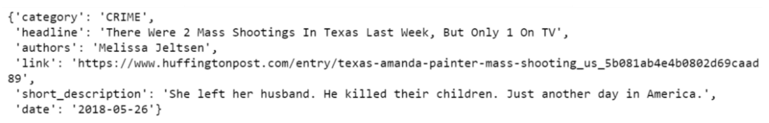

The original dataset contains over 30 categories, but for the purposes of this tutorial, I will work with a subset of 3: Entertainment, Politics, and Tech.

原始数据集包含30多个类别，但是出于本教程的目的，我将使用以下3个子集：娱乐，政治和科技。

## create dtf
dtf = pd.DataFrame(lst_dics)## filter categories
dtf = dtf[ dtf["category"].isin(['ENTERTAINMENT','POLITICS','TECH'])        ][["category","headline"]]## rename columns
dtf = dtf.rename(columns={"category":"y", "headline":"text"})## print 5 random rows
dtf.sample(5)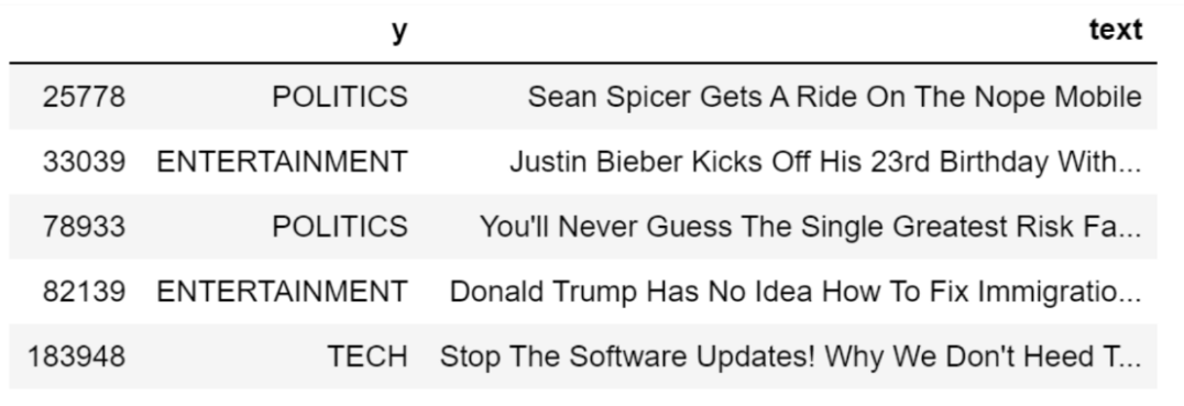

As you can see, the dataset includes a target variable as well. I won’t be using it for modeling, just for performance evaluation.

如您所见，数据集还包含一个目标变量。 我不会将其用于建模，而只是用于性能评估。

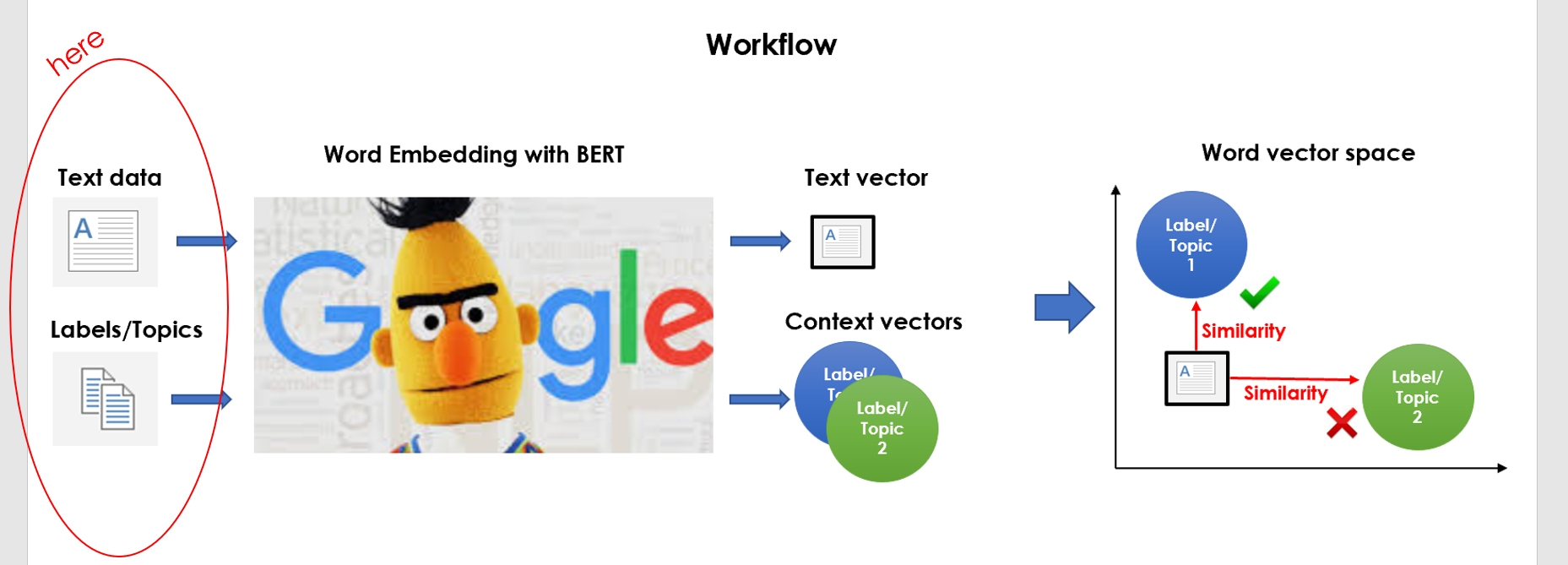
So we’ve got some raw text data and we are tasked to classify it into the 3 categories (Entertainment, Politics, Tech) we know nothing about. Here’s what I am planning to do:

因此，我们获得了一些原始文本数据，并负责将其分类为我们一无所知的3个类别(娱乐，政治，科技)。 这是我打算做的事情：

• clean data and embed it into the vector space,
  清理数据并将其嵌入向量空间，
• create a topic cluster for each category and embed it into the vector space,
  为每个类别创建一个主题集群，并将其嵌入到向量空间中，
• calculate similarities between every text vector and the topic clusters, then assign it to the closest cluster.
  计算每个文本向量与主题簇之间的相似度，然后将其分配给最近的簇。

That is why I called it “a sort of unsupervised text classification”. It’s a really basic idea, but the execution can be tricky.

这就是为什么我称其为“一种无监督的文本分类”。 这是一个非常基本的想法，但是执行起来很棘手。

Now that’s all set, let’s get started.

现在已经准备好了，让我们开始吧。

前处理 (Preprocessing)

The absolute first step is to preprocess the data: cleaning text, removing stop words, and applying lemmatization. I will write a function and apply it to the whole data set.

绝对的第一步是预处理数据：清理文本，删除停用词和应用词形化。 我将编写一个函数并将其应用于整个数据集。

'''
Preprocess a string.
:parameter
    :param text: string - name of column containing text
    :param lst_stopwords: list - list of stopwords to remove
    :param flg_stemm: bool - whether stemming is to be applied
    :param flg_lemm: bool - whether lemmitisation is to be applied
:return
    cleaned text
'''
def utils_preprocess_text(text, flg_stemm=False, flg_lemm=True, lst_stopwords=None):## clean (convert to lowercase and remove punctuations and   
    characters and then strip)
    text = re.sub(r'[^\w\s]', '', str(text).lower().strip())## Tokenize (convert from string to list)
    lst_text = text.split()        ## remove Stopwords
    if lst_stopwords is not None:
        lst_text = [word for word in lst_text if word not in 
                    lst_stopwords]## Stemming (remove -ing, -ly, ...)
    if flg_stemm == True:
        ps = nltk.stem.porter.PorterStemmer()
        lst_text = [ps.stem(word) for word in lst_text]## Lemmatisation (convert the word into root word)
    if flg_lemm == True:
        lem = nltk.stem.wordnet.WordNetLemmatizer()
        lst_text = [lem.lemmatize(word) for word in lst_text]## back to string from list
    text = " ".join(lst_text)
    return text

That function removes a set of words from the corpus if given. I can create a list of generic stop words for the English vocabulary with nltk (we could edit this list by adding or removing words).

该函数会从语料库中删除一组单词(如果有的话)。 我可以使用nltk为英语词汇创建通用停用词的列表(我们可以通过添加或删除单词来编辑此列表)。

lst_stopwords = nltk.corpus.stopwords.words("english")
lst_stopwords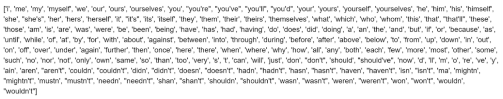

Now I shall apply the function to the whole dataset and store the result in a new column named “text_clean” that I am going to use as a corpus.

现在，我将把函数应用于整个数据集，并将结果存储在名为“ text_clean ”的新列中，该列将用作语料库。

dtf["text_clean"] = dtf["text"].apply(lambda x: utils_preprocess_text(x, flg_stemm=False, flg_lemm=True, lst_stopwords=lst_stopwords))dtf.head()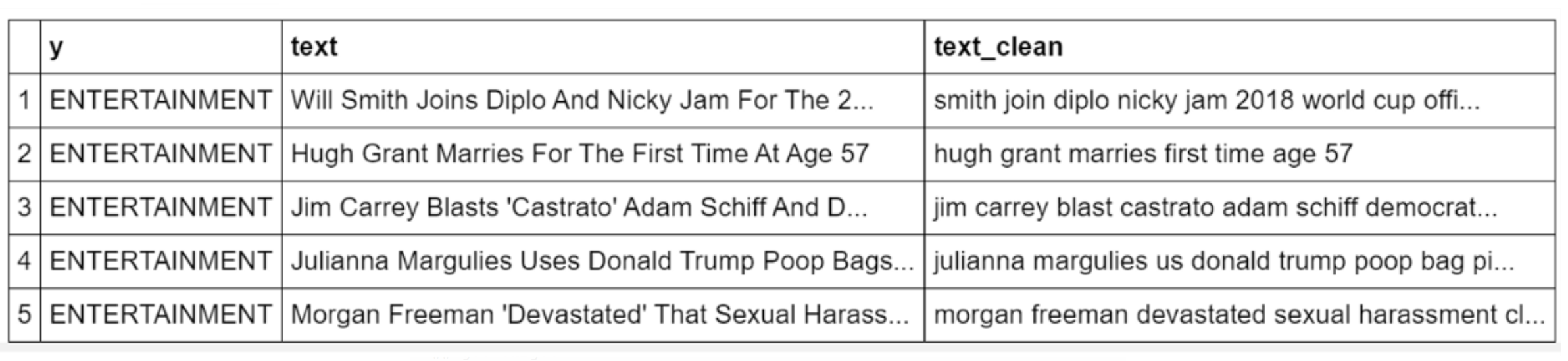

We have our preprocessed corpus, consequently the next step is to build the target variable. Basically, we’re here:

我们有经过预处理的语料库，因此下一步是构建目标变量。 基本上，我们在这里：

创建目标集群 (Create Target Clusters)

The objective of this section is to create some keywords which can represent the context of each category. By performing some text analysis, you can easily discover that the 3 most frequent words are “movie”, “trump”, and “apple” (for a detailed text analysis tutorial you can check this article). I’d suggest starting with those keywords.

本节的目的是创建一些可以表示每个类别的上下文的关键字。 通过执行一些文本分析，您可以轻松发现3个最常见的词是“ 电影 ”，“ 王牌 ”和“ 苹果 ”(有关详细的文本分析教程，您可以查看本文 )。 我建议从这些关键字开始。

Let’s take the Politics category for instance: the word “trump” can have different meanings, so we need to add keywords to avoid polysemy problems (i.e. “donald”, “republican”, “white house”, “obama”). This task could be carried out manually or you could use the assistance of a pre-trained NLP model. You can load a pre-trained Word Embedding model from genism-data like this:

让我们以“政治”类别为例：“ 特朗普 ”一词可能具有不同的含义，因此我们需要添加关键字来避免多义制问题(即“ 唐纳德 ”，“ 共和党 ”，“ 白宫 ”，“ 奥巴马 ”)。 可以手动执行此任务，也可以使用预先训练的NLP模型的帮助。 您可以从genism-data加载预训练的词嵌入模型 像这样：

nlp = gensim_api.load("glove-wiki-gigaword-300")

The gensim package has a very convenient function that returns the most similar words for any given word into the vocabulary.

gensim软件包具有非常方便的功能，该功能可以将任何给定单词的最相似单词返回到词汇表中。

nlp.most_similar(["obama"], topn=3)

I shall use that to create a dictionary of keywords for each category:

我将使用它为每个类别创建一个关键字字典：

## Function to apply
def get_similar_words(lst_words, top, nlp):
    lst_out = lst_words
    for tupla in nlp.most_similar(lst_words, topn=top):
        lst_out.append(tupla[0])
    return list(set(lst_out))## Create Dictionary {category:[keywords]}dic_clusters = {}dic_clusters["ENTERTAINMENT"] = get_similar_words(['celebrity','cinema','movie','music'], 
                  top=30, nlp=nlp)dic_clusters["POLITICS"] = get_similar_words(['gop','clinton','president','obama','republican']
                  , top=30, nlp=nlp)dic_clusters["TECH"] = get_similar_words(['amazon','android','app','apple','facebook',
                   'google','tech'], 
                   top=30, nlp=nlp)## print some
for k,v in dic_clusters.items():
    print(k, ": ", v[0:5], "...", len(v))

Let’s try to visualize those keywords in a 2D space by applying a dimensionality reduction algorithm (i.e. TSNE). We want to make sure that the clusters are well separated from each other.

让我们尝试通过应用降维算法(即TSNE )在2D空间中可视化那些关键字。 我们要确保群集之间的分隔良好。

## word embeddingtot_words = [word for v in dic_clusters.values() for word in v]
X = nlp[tot_words]## pca
pca = manifold.TSNE(perplexity=40, n_components=2, init='pca')
X = pca.fit_transform(X)
## create dtf
dtf = pd.DataFrame()
for k,v in dic_clusters.items():
    size = len(dtf) + len(v)
    dtf_group = pd.DataFrame(X[len(dtf):size], columns=["x","y"], 
                             index=v)
    dtf_group["cluster"] = k
    dtf = dtf.append(dtf_group)## plot
fig, ax = plt.subplots()
sns.scatterplot(data=dtf, x="x", y="y", hue="cluster", ax=ax)ax.legend().texts[0].set_text(None)
ax.set(xlabel=None, ylabel=None, xticks=[], xticklabels=[], 
       yticks=[], yticklabels=[])for i in range(len(dtf)):
    ax.annotate(dtf.index[i], 
               xy=(dtf["x"].iloc[i],dtf["y"].iloc[i]), 
               xytext=(5,2), textcoords='offset points', 
               ha='right', va='bottom')

Cool, they look isolated enough from each other. The Entertainment cluster is closer to the Tech one than the Politics one, which makes sense as words like “apple” and “youtube” can appear in both Tech and Entertainment news.

太酷了，它们看起来彼此足够孤立。 娱乐产业集群比政治产业集群更接近科技集群，这很有意义，因为“ 苹果 ”和“ youtube ”等词可以出现在科技新闻和娱乐新闻中。

特征工程 (Feature Engineering)

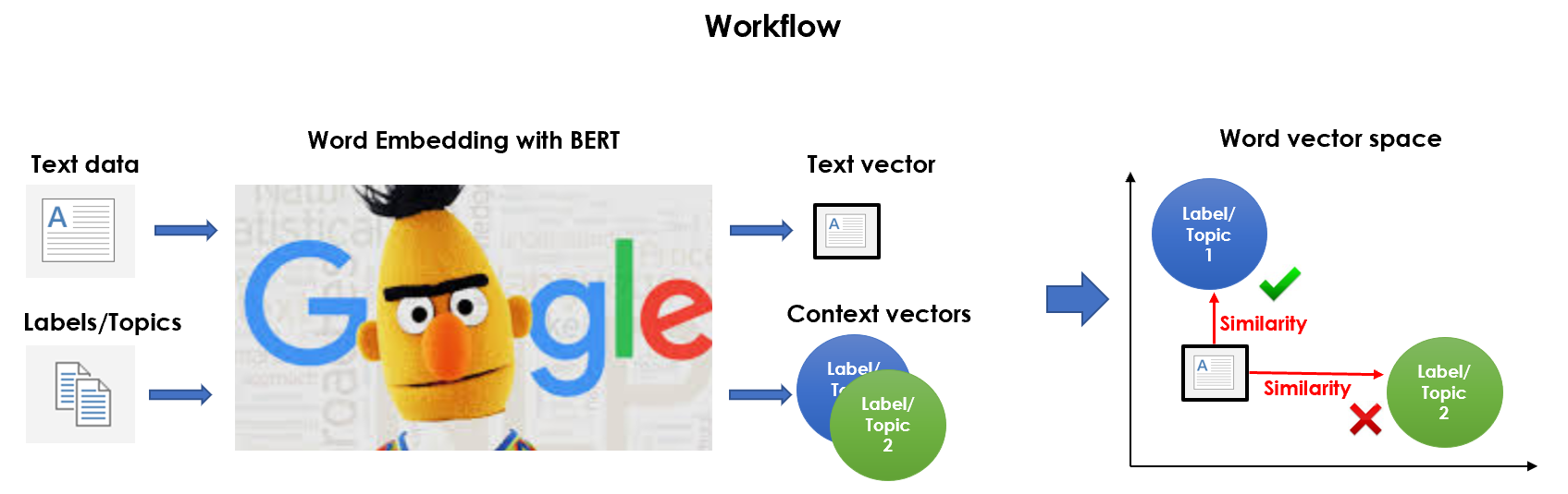
It’s time to embed the corpus we preprocessed and the target clusters we created in the same vector space. Basically, we’re doing this:

现在是时候将我们预处理过的语料库和我们创建的目标聚类嵌入到相同的向量空间中了。 基本上，我们正在这样做：

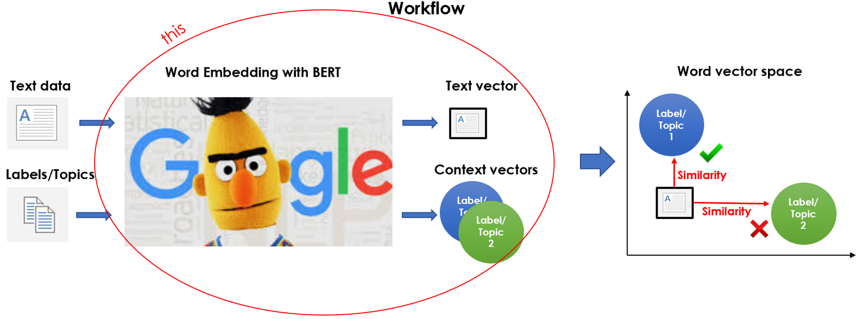
Yes, I’m using BERT for this. It’s true that you could utilize any Word Embedding model (i.e. Word2Vec, Glove, …), even the one that we already loaded to define keywords, so why bother to use such a heavy and complex language model? That’s because BERT doesn’t apply a fixed embedding, instead it looks at the entire sentence and then assigns an embedding to each word. Therefore, the vector BERT assigns to a word is a function of the entire sentence, so that a word can have different vectors based on the contexts.

是的，我正在为此使用BERT 。 的确，您可以利用任何Word嵌入模型(即Word2Vec，Glove等)，甚至可以使用我们已经加载的用于定义关键字的模型，那么，为什么要麻烦使用这么繁琐的语言模型呢？ 这是因为BERT不会应用固定的嵌入，而是会查看整个句子，然后为每个单词分配一个嵌入。 因此，BERT分配给单词的向量是整个句子的函数，因此单词可以基于上下文具有不同的向量。

I’m going to load the original pre-trained version of BERT with the package transformers and give an example of the dynamic embedding:

我将使用软件包转换器加载BERT的原始预训练版本，并提供动态嵌入的示例：

tokenizer = transformers.BertTokenizer.from_pretrained('bert-base-
            uncased', do_lower_case=True)nlp = transformers.TFBertModel.from_pretrained('bert-base-uncased')

Let’s use the model to convert the string “river bank” into vectors and print the one assigned to the word “bank”:

让我们使用该模型将字符串“ river bank ”转换为向量，并打印分配给单词“ bank ”的那个：

txt = "river bank"## tokenize
idx = tokenizer.encode(txt)
print("tokens:", tokenizer.convert_ids_to_tokens(idx))
print("ids   :", tokenizer.encode(txt))## word embedding
idx = np.array(idx)[None,:]
embedding = nlp(idx)
print("shape:", embedding[0][0].shape)## vector of the second input word
embedding[0][0][2]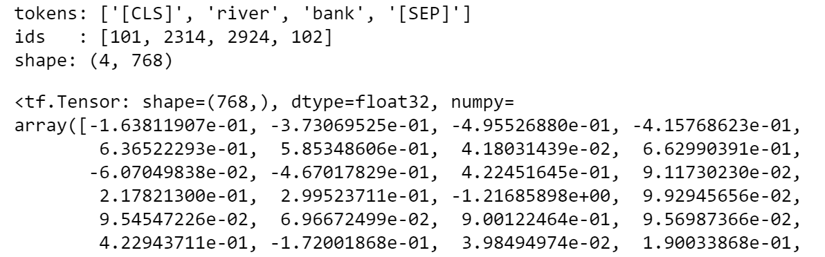

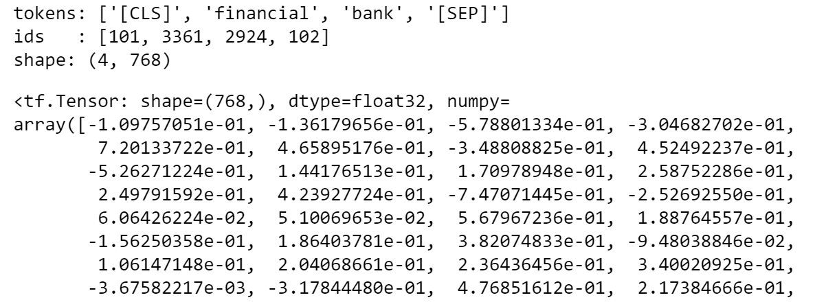
If you do the same for the string “financial bank”, you’ll see that the vector assigned to the word “bank” is different because of the context. Please note that the BERT tokenizer inserts special tokens at the beginning and end of sentences and its vector space has a dimension of 768 (to understand better how BERT processes text you can check this article).

如果对字符串“ financial bank ”执行相同的操作，则会发现分配给单词“ bank ”的向量因上下文而不同。 请注意，BERT令牌生成器在句子的开头和结尾插入特殊的令牌，其向量空间的尺寸为768(要更好地了解BERT如何处理文本，您可以查看本文 )。

Having said that, the plan is to use BERT Word Embedding to represent each text with an array (shape: number of tokens x 768) and then summarize each article into a mean vector.

话虽如此，我们的计划是使用BERT词嵌入法以数组(形状：令牌数x 768)表示每个文本，然后将每个文章汇总为均值向量。

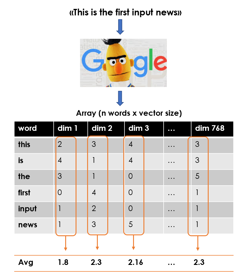
So the final feature matrix will be an array with shape: number of documents (or mean vectors) x 768.

因此，最终的特征矩阵将是一个具有以下形状的数组：文档数(或均值向量)x 768。

## function to applydef utils_bert_embedding(txt, tokenizer, nlp):
    idx = tokenizer.encode(txt)
    idx = np.array(idx)[None,:]  
    embedding = nlp(idx)
    X = np.array(embedding[0][0][1:-1])
    return X## create list of news vector
lst_mean_vecs = [utils_bert_embedding(txt, tokenizer, nlp).mean(0) 
                 for txt in x]## create the feature matrix (n news x 768)
X = np.array(lst_mean_vecs)

We can do the same with the keywords in the target clusters. In fact, each label is identified by a list of words that help BERT to understand the context within the clusters. Hence, I’m going to create a dictionary label : cluster mean vector.

我们可以对目标集群中的关键字执行相同的操作。 实际上，每个标签都由一系列单词来标识，这些单词可以帮助BERT理解群集中的上下文。 因此，我将创建一个字典标签：簇均值向量。

dic_y = {k:utils_bert_embedding(v, tokenizer, nlp).mean(0) for k,v
         in dic_clusters.items()}

We started with just some text data and 3 strings (“Entertainment”, “Politics”, “Tech”) and now we have a feature matrix and a target variable… ish.

我们仅从一些文本数据和3个字符串( “娱乐”，“政治”，“技术” )开始，现在我们有了一个特征矩阵和一个目标变量……ish。

模型设计与测试 (Model Design & Testing)

Finally, it’s time to build a model that classifies the news based on the similarity to each target cluster.

最后，是时候建立一个模型，根据与每个目标集群的相似性对新闻进行分类。

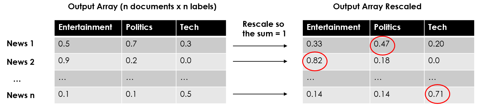
I am going to use Cosine Similarity, a measure of similarity based on the cosine of the angle between two non-zero vectors, which equals the inner product of the same vectors normalized to both have length 1. You can easily use the cosine similarity implementation of scikit-learn, which takes 2 arrays (or vectors) and returns an array of scores (or a single score). In this case, the output is going to be a matrix with shape: number of news x number of labels (3, Entertainment/Politics/Tech). To put it another way, each row will represent an article and contain one similarity score for each target cluster.

我将使用余弦相似度 ，一种基于两个非零向量之间夹角的余弦的相似度度量，它等于归一化为长度为1的相同向量的内积。您可以轻松地使用余弦相似度实现scikit-learn的值 ，它采用2个数组(或向量)并返回一个分数数组(或单个分数)。 在这种情况下，输出将是一个具有以下形状的矩阵：新闻数量x标签数量(3，娱乐/政治/科技)。 换句话说，每一行将代表一篇文章，并为每个目标聚类包含一个相似性得分。

In order to run the usual evaluation metrics (Accuracy, AUC, Precision, Recall, …), we have to rescale the scores in each row so that they sum to 1 and decide a category to label the article with. I’m going to choose the one with the highest score, but it could be wise to set some minimum thresholds and leave out predictions with really low scores.

为了运行常用的评估指标(准确性，AUC，精度，召回率，...)，我们必须重新调整每行中的得分，使它们的总和为1，并确定用于标记文章的类别。 我将选择得分最高的那个，但设置一些最小阈值并忽略得分非常低的预测可能是明智的。

#--- Model Algorithm ---### compute cosine similarities
similarities = np.array(
            [metrics.pairwise.cosine_similarity(X, y).T.tolist()[0] 
             for y in dic_y.values()]
            ).T## adjust and rescale
labels = list(dic_y.keys())
for i in range(len(similarities)):    ### assign randomly if there is no similarity
    if sum(similarities[i]) == 0:
       similarities[i] = [0]*len(labels)
       similarities[i][np.random.choice(range(len(labels)))] = 1    ### rescale so they sum = 1
    similarities[i] = similarities[i] / sum(similarities[i])
## classify the label with highest similarity scorepredicted_prob = similarities
predicted = [labels[np.argmax(pred)] for pred in predicted_prob]

Just like in classic supervised use cases, we have an object with predicted probabilities (here they’re adjusted similarity scores) and another with predicted labels. Let’s check how we did:

就像在经典的监督用例中一样，我们有一个对象具有预测的概率(在此情况下，它们是经过调整的相似性评分)，而另一个对象则具有预测的标签。 让我们检查一下如何做：

y_test = dtf["y"].values
classes = np.unique(y_test)
y_test_array = pd.get_dummies(y_test, drop_first=False).values
## Accuracy, Precision, Recall
accuracy = metrics.accuracy_score(y_test, predicted)
auc = metrics.roc_auc_score(y_test, predicted_prob, 
                            multi_class="ovr")
print("Accuracy:",  round(accuracy,2))
print("Auc:", round(auc,2))
print("Detail:")
print(metrics.classification_report(y_test, predicted))## Plot confusion matrix
cm = metrics.confusion_matrix(y_test, predicted)
fig, ax = plt.subplots()
sns.heatmap(cm, annot=True, fmt='d', ax=ax, cmap=plt.cm.Blues, 
            cbar=False)
ax.set(xlabel="Pred", ylabel="True", xticklabels=classes, 
       yticklabels=classes, title="Confusion matrix")
plt.yticks(rotation=0)
fig, ax = plt.subplots(nrows=1, ncols=2)
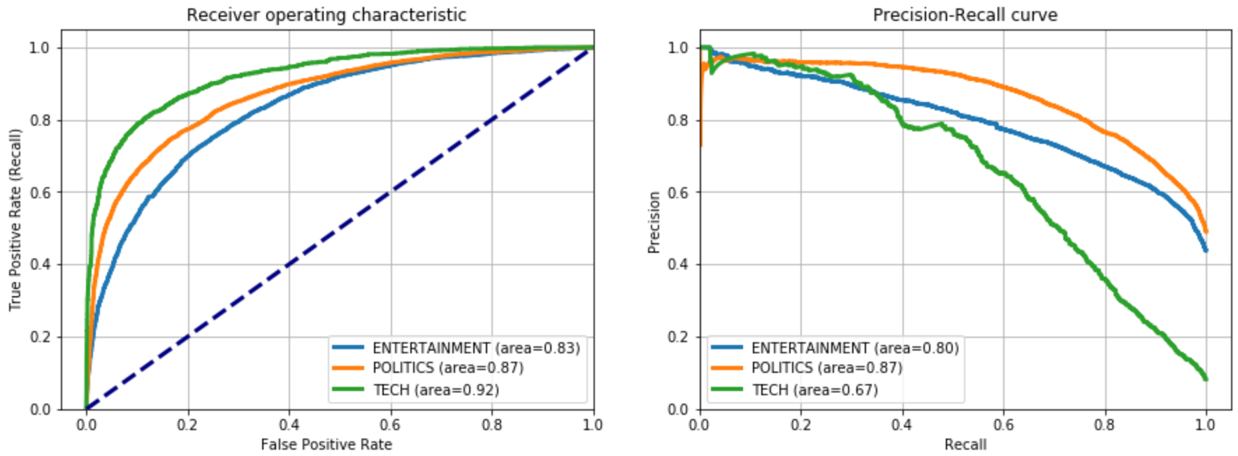
## Plot roc
for i in range(len(classes)):
    fpr, tpr, thresholds = metrics.roc_curve(y_test_array[:,i],  
                           predicted_prob[:,i])
    ax[0].plot(fpr, tpr, lw=3, 
              label='{0} (area={1:0.2f})'.format(classes[i], 
                              metrics.auc(fpr, tpr))
               )
ax[0].plot([0,1], [0,1], color='navy', lw=3, linestyle='--')
ax[0].set(xlim=[-0.05,1.0], ylim=[0.0,1.05], 
          xlabel='False Positive Rate', 
          ylabel="True Positive Rate (Recall)", 
          title="Receiver operating characteristic")
ax[0].legend(loc="lower right")
ax[0].grid(True)## Plot precision-recall curvefor i in range(len(classes)):
    precision, recall, thresholds = metrics.precision_recall_curve(
                 y_test_array[:,i], predicted_prob[:,i])
    ax[1].plot(recall, precision, lw=3, 
               label='{0} (area={1:0.2f})'.format(classes[i], 
                                  metrics.auc(recall, precision))
              )
ax[1].set(xlim=[0.0,1.05], ylim=[0.0,1.05], xlabel='Recall', 
          ylabel="Precision", title="Precision-Recall curve")
ax[1].legend(loc="best")
ax[1].grid(True)
plt.show()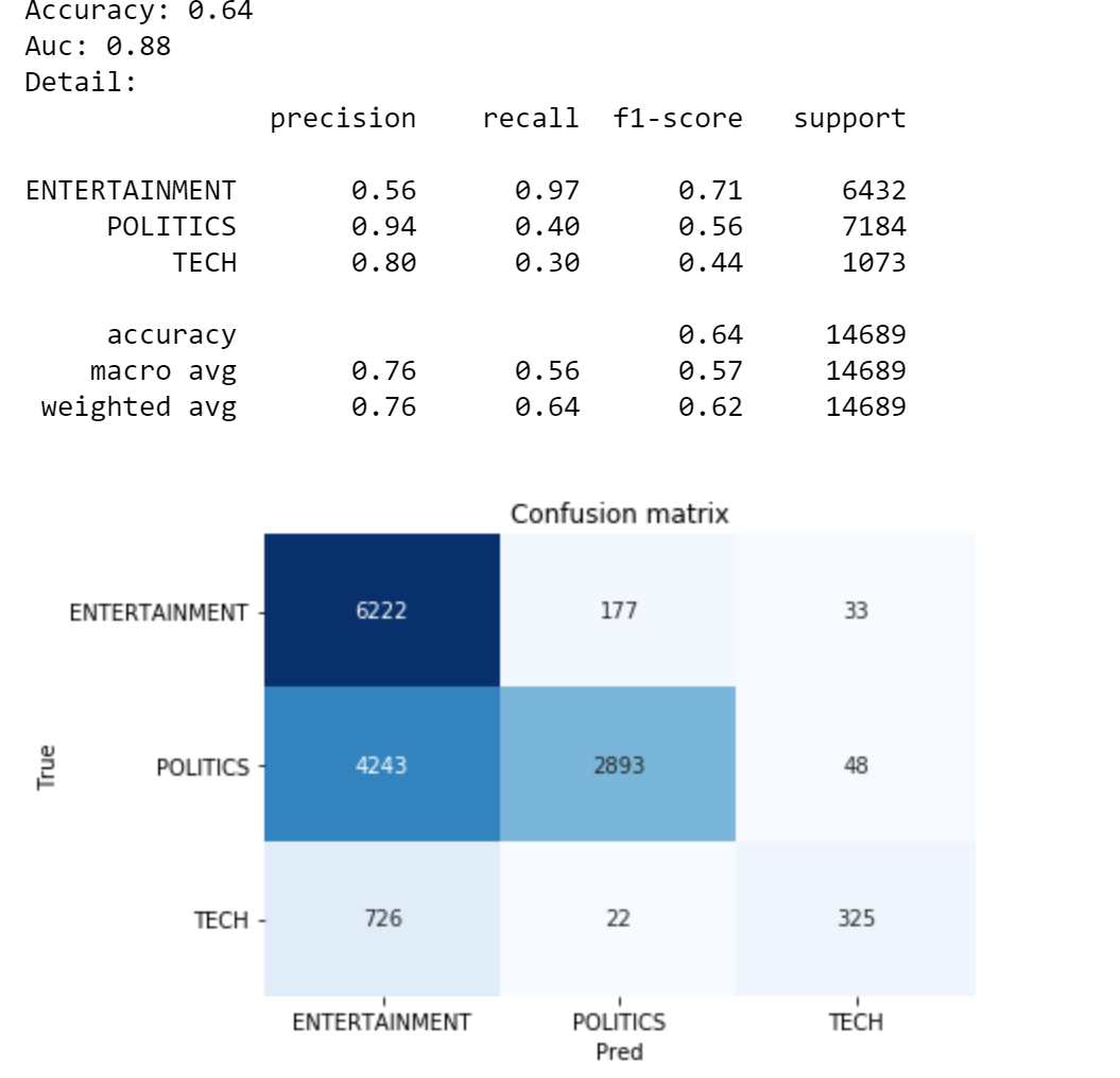

Okay, I’m the first to say that it’s not the best Accuracy I’ve ever seen. On the other hand, it’s not bad at all considering that we didn’t train any model and we even made up the target variable. The main issue is over 4k Politics observations classified as Entertainment, but these performances can be easily improved by fine-tuning the keywords for those two categories.

好的，我是第一个说这不是我见过的最好的准确性。 另一方面，考虑到我们没有训练任何模型甚至我们组成了目标变量，这一点也不错。 主要问题是分类为“娱乐”的4k Politics观察结果，但是通过微调这两个类别的关键字，可以轻松提高这些性能。

可解释性 (Explainability)

Let’s try to understand what led our algorithm to classify news with a category instead of the others. Let’s take a random observation from the corpus:

让我们尝试了解是什么导致我们的算法将新闻按类别而不是其他类别进行分类。 让我们从语料库中随机观察：

i = 7txt_instance = dtf["text_clean"].iloc[i]print("True:", y_test[i], "--> Pred:", predicted[i], "| 
      Similarity:", round(np.max(predicted_prob[i]),2))
print(txt_instance)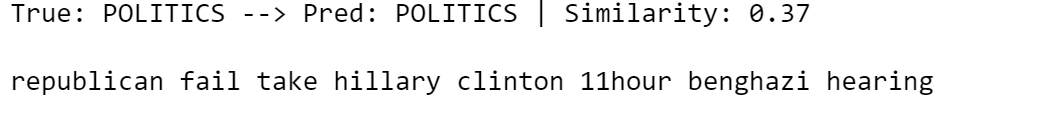

It’s a Politics observation properly classified. Probably, the words “republican” and “clinton” gave BERT the right hint. I will visualize the mean vector of the article in a 2D space and plot the top similarities with the target cluster.

这是对政治观察的正确分类。 可能“ 共和党 ”和“ 克林顿 ”这两个词给了BERT正确的提示。 我将在2D空间中可视化文章的均值向量，并绘制与目标簇的顶级相似性。

## create embedding Matrixy = np.concatenate([embedding_bert(v, tokenizer, nlp) for v in 
                    dic_clusters.values()])
X = embedding_bert(txt_instance, tokenizer,
                   nlp).mean(0).reshape(1,-1)
M = np.concatenate([y,X])
## pca
pca = manifold.TSNE(perplexity=40, n_components=2, init='pca')
M = pca.fit_transform(M)
y, X = M[:len(y)], M[len(y):]
## create dtf clusters
dtf = pd.DataFrame()
for k,v in dic_clusters.items():
    size = len(dtf) + len(v)
    dtf_group = pd.DataFrame(y[len(dtf):size], columns=["x","y"], 
                             index=v)
    dtf_group["cluster"] = k
    dtf = dtf.append(dtf_group)
## plot clusters
fig, ax = plt.subplots()
sns.scatterplot(data=dtf, x="x", y="y", hue="cluster", ax=ax)
ax.legend().texts[0].set_text(None)
ax.set(xlabel=None, ylabel=None, xticks=[], xticklabels=[], 
       yticks=[], yticklabels=[])
for i in range(len(dtf)):
    ax.annotate(dtf.index[i], 
               xy=(dtf["x"].iloc[i],dtf["y"].iloc[i]), 
               xytext=(5,2), textcoords='offset points', 
               ha='right', va='bottom')
## add txt_instanceax.scatter(x=X[0][0], y=X[0][1], c="red", linewidth=10)
           ax.annotate("x", xy=(X[0][0],X[0][1]), 
           ha='center', va='center', fontsize=25)
## calculate similaritysim_matrix = metrics.pairwise.cosine_similarity(X, y)
## add top similarity
for row in range(sim_matrix.shape[0]):    ### sorted {keyword:score}
    dic_sim = {n:sim_matrix[row][n] for n in 
               range(sim_matrix.shape[1])}
    dic_sim = {k:v for k,v in sorted(dic_sim.items(), 
                key=lambda item:item[1], reverse=True)}    ### plot lines
    for k in dict(list(dic_sim.items())[0:5]).keys():
        p1 = [X[row][0], X[row][1]]
        p2 = [y[k][0], y[k][1]]
        ax.plot([p1[0],p2[0]], [p1[1],p2[1]], c="red", alpha=0.5)plt.show()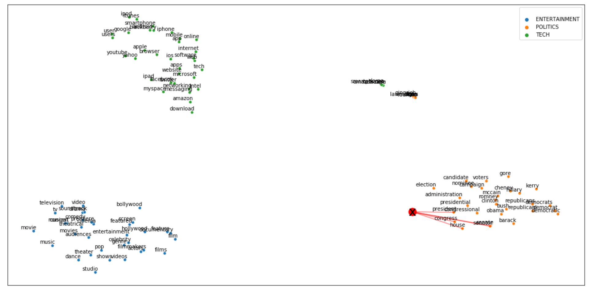

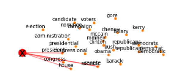
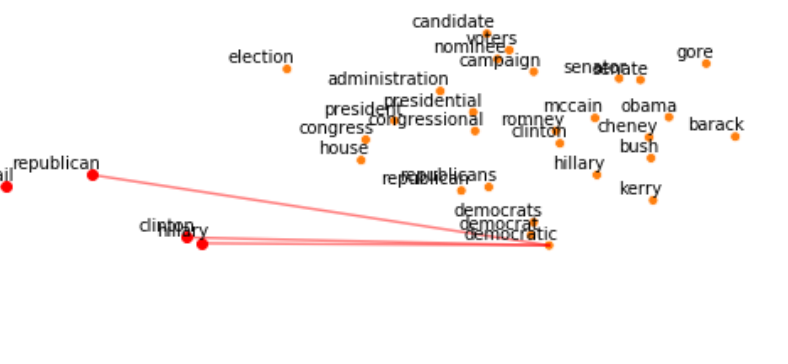
Let’s zoom a bit on the cluster of interest:

让我们放大一下感兴趣的集群：

Overall, we can say the mean vector is pretty similar to the Politics cluster. Let’s break down the article into tokens to see which ones “activated” the right cluster.

总体而言，我们可以说均值向量与Politics集群非常相似。 让我们将文章分解为令牌，以查看哪些令牌“激活”了正确的群集。

## create embedding Matrixy = np.concatenate([embedding_bert(v, tokenizer, nlp) for v in 
                    dic_clusters.values()])
X = embedding_bert(txt_instance, tokenizer,
                   nlp).mean(0).reshape(1,-1)
M = np.concatenate([y,X])
## pca
pca = manifold.TSNE(perplexity=40, n_components=2, init='pca')
M = pca.fit_transform(M)
y, X = M[:len(y)], M[len(y):]
## create dtf clusters
dtf = pd.DataFrame()
for k,v in dic_clusters.items():
    size = len(dtf) + len(v)
    dtf_group = pd.DataFrame(y[len(dtf):size], columns=["x","y"], 
                             index=v)
    dtf_group["cluster"] = k
    dtf = dtf.append(dtf_group)
## add txt_instancetokens = tokenizer.convert_ids_to_tokens(
               tokenizer.encode(txt_instance))[1:-1]
dtf = pd.DataFrame(X, columns=["x","y"], index=tokens)
dtf = dtf[~dtf.index.str.contains("#")]
dtf = dtf[dtf.index.str.len() > 1]
X = dtf.values
ax.scatter(x=dtf["x"], y=dtf["y"], c="red")
for i in range(len(dtf)):
     ax.annotate(dtf.index[i], 
                 xy=(dtf["x"].iloc[i],dtf["y"].iloc[i]), 
                 xytext=(5,2), textcoords='offset points', 
                 ha='right', va='bottom')
## calculate similaritysim_matrix = metrics.pairwise.cosine_similarity(X, y)
## add top similarity
for row in range(sim_matrix.shape[0]):    ### sorted {keyword:score}
    dic_sim = {n:sim_matrix[row][n] for n in 
               range(sim_matrix.shape[1])}
    dic_sim = {k:v for k,v in sorted(dic_sim.items(), 
                key=lambda item:item[1], reverse=True)}    ### plot lines
    for k in dict(list(dic_sim.items())[0:5]).keys():
        p1 = [X[row][0], X[row][1]]
        p2 = [y[k][0], y[k][1]]
        ax.plot([p1[0],p2[0]], [p1[1],p2[1]], c="red", alpha=0.5)plt.show()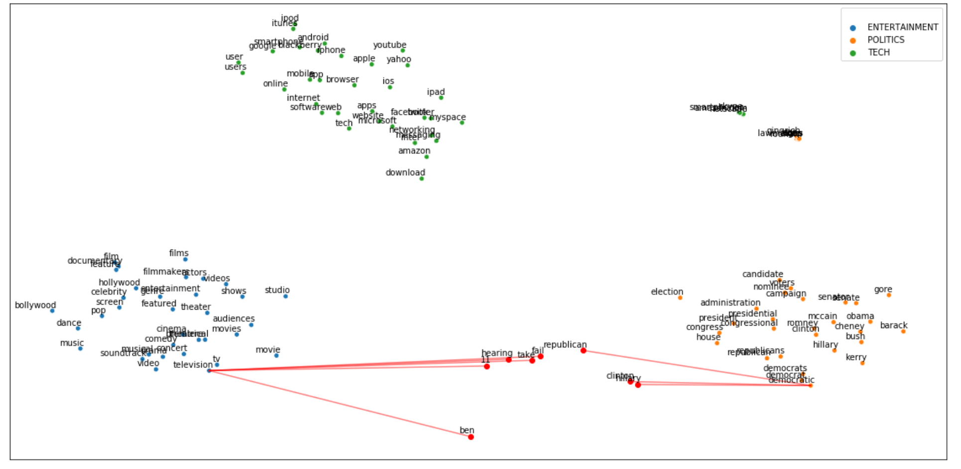

As we thought, there are words in the text which are clearly linked to the Politics cluster, but some others are more similar to the Entertainment general context.

正如我们所认为的，文本中有一些单词与“政治”类明显相关，但其他一些单词与“娱乐”的一般上下文更为相似。

结论 (Conclusion)

This article has been a tutorial to demonstrate how to perform text classification when a labeled training set isn't available.

本文是一个教程，以演示在没有标签训练集的情况下如何进行文本分类 。

I used a pre-trained Word Embedding model to build a set of keywords to contextualize the target variable. Then I transformed those words and the corpus in the same vector space with the pre-trained BERT language model. Finally, I calculated the Cosine Similarity between text and keywords to determine the context of each article and I used that information to label the news.

我使用了预训练的单词嵌入模型来构建一组关键字，以将目标变量关联起来。 然后，我使用预先训练的BERT语言模型在相同的向量空间中转换了这些单词和语料库。 最后，我计算了文本和关键字之间的余弦相似度，以确定每篇文章的上下文，然后使用该信息来标记新闻。

This strategy isn’t the most effective but it’s definitely efficient as it allows you to deliver good results quickly. Moreover, this algorithm can be used as a baseline for a supervised model, once a labeled dataset is obtained.

该策略不是最有效的，但绝对有效，因为它可以使您快速交付良好的结果。 此外，一旦获得标记的数据集，该算法就可以用作监督模型的基线。

This article is part of the series NLP with Python, see also:

本文是 Python 系列 NLP的 一部分 ，另请参见：

Contacts: LinkedIn | Twitter

联系人： 领英 | 推特