OpenGL学习脚印: 投影矩阵和视口变换矩阵(math-projection and viewport matrix)

写在前面前面几节分别介绍了模型变换，视变换，本节继续学习OpenGL坐标变换过程中的投影变换。这里主要是从数学角度推导投影矩阵。对数学不感兴趣的，可以稍微了解下，或者跳过本节内容。本文主要翻译并整理自 songho OpenGL Projection Matrix一文，这里对他的推导思路稍微进行了整理。通过本节可以了解到透视投影矩阵的推导正交投影矩阵的推导视口变换矩阵的推导zF

The fool

48969人浏览 · 2016-06-05 18:06:42

The fool · 2016-06-05 18:06:42 发布

写在前面
前面几节分别介绍了模型变换，视变换，本节继续学习OpenGL坐标变换过程中的投影变换。这里主要是从数学角度推导投影矩阵。对数学不感兴趣的，可以稍微了解下，或者跳过本节内容。

本文主要翻译并整理自 songho OpenGL Projection Matrix一文，这里对他的推导思路稍微进行了整理。

通过本节可以了解到

透视投影矩阵的推导
正交投影矩阵的推导
视口变换矩阵的推导
zFighting问题

投影变换

OpenGL最终的渲染设备是2D的，我们需要将3D表示的场景转换为最终的2D形式，前面使用模型变换和视变换将物体坐标转换到照相机坐标系后，需要进行投影变换，将坐标从相机—》裁剪坐标系，经过透视除法后，变换到规范化设备坐标系(NDC)，最后进行视口变换后，3D坐标才变换到屏幕上的2D坐标，这个过程如下图所示：

坐标变换

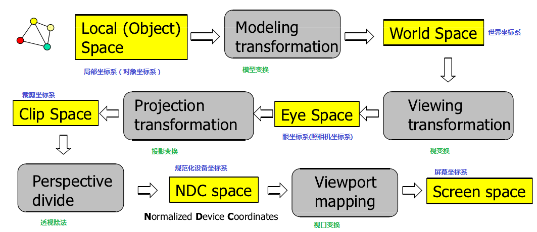
投影变换通过指定视见体(viewing frustum)来决定场景中哪些物体将可能会呈现在屏幕上。在视见体中的物体会出现在投影平面上，而在视见体之外的物体不会出现在投影平面上。投影包括很多类型，OpenGL中主要考虑透视投影(perspective projection)和正交投影( orthographic projection)。两者之间存在很大的区别，如下图所示(图片来自Modern OpenGL)：

投影类型

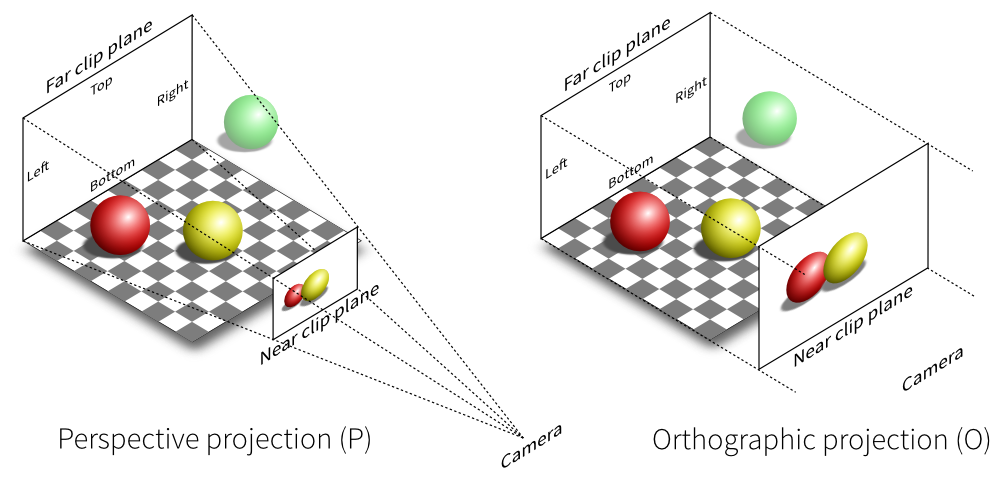
上面的图中，红色和黄色球在视见体内，因而呈现在投影平面上，而绿色球在视见体外，没有在投影平面上成像。

指定视见体通过(GLdouble left, GLdouble right, GLdouble bottom, GLdouble top, GLdouble nearVal, GLdouble farVal)6个参数来指定。注意在相机坐标系下，相机指向-z轴，nearVal和farVal表示的剪裁平面分别为:近裁剪平面 z=−nearVal <script id="MathJax-Element-1" type="math/tex">z = -nearVal</script>，以及远裁剪平面 z=−farVal <script id="MathJax-Element-2" type="math/tex">z = -farVal</script>。推导投影矩阵，就要利用这6个参数。在OpenGL中成像是在近裁剪平面上完成。

透视投影矩阵的推导

透视投影中，相机坐标系中点被映射到一个标准立方体中，即规范化设备坐标系中，其中 [l,r]映射到[−1,1] <script id="MathJax-Element-3" type="math/tex">[l,r]映射到[-1,1]</script>， [b,t] <script id="MathJax-Element-4" type="math/tex">[b,t]</script>映射到[-1,1]中，以及 [n,f] <script id="MathJax-Element-5" type="math/tex">[n,f]</script>被映射到 [−1,1] <script id="MathJax-Element-6" type="math/tex">[-1,1]</script>，如下图所示：
视见体和NDC

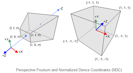
注意到上面的相机坐标系为右手系，而NDC中+z轴向内，为左手系。

我们的目标

求出投影矩阵的目标就是要找到一个透视投影矩阵P使得下式成立：

⎡ ⎣ ⎢ ⎢ ⎢ x c y c z c w c ⎤ ⎦ ⎥ ⎥ ⎥ = P * ⎡ ⎣ ⎢ ⎢ ⎢ x e y e z e w e ⎤ ⎦ ⎥ ⎥ ⎥

⎡ ⎣ ⎢ x n y n z n ⎤ ⎦ ⎥ = ⎡ ⎣ ⎢ x c / w c y c / w c z c / w c ⎤ ⎦ ⎥

wclip <script id="MathJax-Element-9" type="math/tex">w_{clip}</script>过程被称为透视除法。要找到我们需要的矩阵P，我们需要利用两个关系:

投影位置 xp <script id="MathJax-Element-10" type="math/tex">x_{p}</script>, yp <script id="MathJax-Element-11" type="math/tex">y_{p}</script>和相机坐标系中点 xe <script id="MathJax-Element-12" type="math/tex">x_{e}</script>, ye之间关系。投影后对于z分量都是 <script id="MathJax-Element-13" type="math/tex">y_{e}之间关系。投影后对于z分量都是</script>z_{p}=-nearVal$。
利用 xp <script id="MathJax-Element-14" type="math/tex">x_{p}</script>， yp <script id="MathJax-Element-15" type="math/tex">y_{p}</script>和 xndc，yndc <script id="MathJax-Element-16" type="math/tex">x_{ndc}，y_{ndc}</script>关系求出 xclip,yclip <script id="MathJax-Element-17" type="math/tex">x_{clip},y_{clip}</script>。
利用 zn <script id="MathJax-Element-18" type="math/tex">z_{n}</script>与 ze <script id="MathJax-Element-19" type="math/tex">z_{e}</script>关系得出 zclip <script id="MathJax-Element-20" type="math/tex">z_{clip}</script>

计算投影平面上的位置

投影时原先位于相机坐标系中的点 p=(xe,ye,ze) <script id="MathJax-Element-3852" type="math/tex">p=(x_{e},y_{e},z_{e})</script>投影到投影平面后，得到点 p′=(xp,yp,−nearVal) <script id="MathJax-Element-3853" type="math/tex">p'=(x_{p},y_{p},-nearVal)</script>。具体过程如下图所示：
投影平面上的点

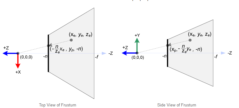
需要空间想象一下，可以得出左边的图是俯视图，右边是侧视图。
利用三角形的相似性，通过俯视图可以计算得到:
xpxe=−nze <script id="MathJax-Element-3854" type="math/tex">\frac{x_{p}}{x_{e}} = \frac{-n}{z_{e}}</script>
即: xp=xen−ze(1.1) <script id="MathJax-Element-3855" type="math/tex">x_{p} = \frac{x_{e}n}{-z_{e}} \tag{1.1}</script>
同理通过侧视图可以得到：
yp=yen−ze(1.2) <script id="MathJax-Element-3856" type="math/tex">y_{p} = \frac{y_{e}n}{-z_{e}}\tag{1.2}</script>

由(1)(2)这个式子可以发现，他们都除以了 −ze <script id="MathJax-Element-3857" type="math/tex">-z_{e}</script>这个量，并且与之成反比。这可以作为透视除法的一个线索，因此我们的矩阵P的形式如下：

⎡ ⎣ ⎢ ⎢ ⎢ x c y c z c w c ⎤ ⎦ ⎥ ⎥ ⎥ = ⎡ ⎣ ⎢ ⎢ ⎢ . . . 0 . . . 0 . . . - 1 . . . 0 ⎤ ⎦ ⎥ ⎥ ⎥ * ⎡ ⎣ ⎢ ⎢ ⎢ x e y e z e w e ⎤ ⎦ ⎥ ⎥ ⎥

wc=−ze <script id="MathJax-Element-3859" type="math/tex">w_{c} = -z_{e}</script>。
下面利用投影点和规范化设备坐标的关系计算出矩阵P的前面两行。
对于投影平面上

xp <script id="MathJax-Element-3860" type="math/tex">x_{p}</script>满足

[l,r] <script id="MathJax-Element-3861" type="math/tex">[l,r]</script>线性映射到

[−1,1] <script id="MathJax-Element-3862" type="math/tex">[-1,1]</script>对于

yp <script id="MathJax-Element-3863" type="math/tex">y_{p}</script>满足

[b,t] <script id="MathJax-Element-3864" type="math/tex">[b,t]</script>线性映射到

[−1,1] <script id="MathJax-Element-3865" type="math/tex">[-1,1]</script>。

其中 xp <script id="MathJax-Element-3866" type="math/tex">x_{p}</script>的映射关系如下图所示：

投影点xp线性映射

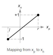
则可以得到 xp <script id="MathJax-Element-3867" type="math/tex">x_{p}</script>的线性关系：
xn=2r−lxp+β(1.3) <script id="MathJax-Element-3868" type="math/tex">x_{n} = \frac{2}{r - l}x_{p}+\beta \tag{1.3}</script>
将(r,1)带入上式得到：
β=−r+lr−l <script id="MathJax-Element-3869" type="math/tex">\beta = -\frac{r+l}{r-l}</script>
带入式子3得到：
xn=2r−lxp−r+lr−l(1.4) <script id="MathJax-Element-3870" type="math/tex">x_{n} = \frac{2}{r - l}x_{p} -\frac{r+l}{r-l} \tag{1.4}</script>
将式子1带入式子5得到：

x n = 2 x e n r - l * 1 - z e - r + l r - l = ( 2 x e n r - l + r + l r - l * z e ) - z e (1.5)

由式子6可以得到:
xc=2nr−lxe+r+lr−l∗ze(1.6) <script id="MathJax-Element-3872" type="math/tex">x_{c} =\frac{2n}{r - l}x_{e}+\frac{r+l}{r-l}*z_{e} \tag{1.6} </script>

对于 yp <script id="MathJax-Element-3873" type="math/tex">y_{p}</script>的映射关系如下：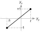
投影点yp线性映射
同理也可以计算得到:

y n = 2 y e n t - b * 1 - z e - t + b t - b = ( 2 y e n t - b + t + b t - b * z e ) - z e (1.7)

yc=2nt−bye+t+bt−b∗ze(1.8) <script id="MathJax-Element-3875" type="math/tex">y_{c} =\frac{2n}{t - b}y_{e}+\frac{t+b}{t-b}*z_{e} \tag{1.8} </script>

由式子7和9可以得到矩阵P的前两行和第四行为：

⎡ ⎣ ⎢ ⎢ ⎢ x c y c z c w c ⎤ ⎦ ⎥ ⎥ ⎥ = ⎡ ⎣ ⎢ ⎢ ⎢ ⎢ ⎢ ⎢ ⎢ 2 n r - l 0.0 0 2 n t - b . 0 r + l r - l t + b t - b . - 1 00.0 ⎤ ⎦ ⎥ ⎥ ⎥ ⎥ ⎥ ⎥ ⎥ * ⎡ ⎣ ⎢ ⎢ ⎢ x e y e z e w e ⎤ ⎦ ⎥ ⎥ ⎥

由于 ze <script id="MathJax-Element-3877" type="math/tex">z_{e}</script>投影到平面时结果都为 −n <script id="MathJax-Element-3878" type="math/tex">-n</script>，因此寻找 zn <script id="MathJax-Element-3879" type="math/tex">z_{n}</script>与之前的x,y分量不太一样。我们知道 zn <script id="MathJax-Element-3880" type="math/tex">z_{n}</script>与x,y分量无关，因此上述矩阵P可以书写为：

⎡ ⎣ ⎢ ⎢ ⎢ x c y c z c w c ⎤ ⎦ ⎥ ⎥ ⎥ = ⎡ ⎣ ⎢ ⎢ ⎢ ⎢ ⎢ ⎢ ⎢ 2 n r - l 000 0 2 n t - b 00 r + l r - l t + b t - b A - 1 00 B 0 ⎤ ⎦ ⎥ ⎥ ⎥ ⎥ ⎥ ⎥ ⎥ * ⎡ ⎣ ⎢ ⎢ ⎢ x e y e z e w e ⎤ ⎦ ⎥ ⎥ ⎥

则有： zn=Aze+Bwe−ze <script id="MathJax-Element-3882" type="math/tex">z_{n} = \frac{Az_{e}+Bw_{e}}{-z_{e}}</script>,由于相机坐标系中 we=1 <script id="MathJax-Element-3883" type="math/tex">w_{e} = 1</script>，则可以进一步书写为：
zn=Aze+B−ze(1.9) <script id="MathJax-Element-3884" type="math/tex">z_{n} = \frac{Az_{e}+B}{-z_{e}} \tag{1.9}</script>

要求出系数A,B则，利用 zn <script id="MathJax-Element-3885" type="math/tex">z_{n}</script>与 ze <script id="MathJax-Element-3886" type="math/tex">z_{e}</script>的映射关系为：(-n，-1)和(-f,1)，代入式子10得到：
A=−f+nf−n <script id="MathJax-Element-3887" type="math/tex">A =-\frac{f+n}{f-n}</script>和 B=−2fnf−n <script id="MathJax-Element-3888" type="math/tex">B= -\frac{2fn}{f-n}</script>，
则 zn <script id="MathJax-Element-3889" type="math/tex">z_{n}</script>与 ze <script id="MathJax-Element-3890" type="math/tex">z_{e}</script>的关系式表示为：
zn=−f+nf−nze−2fnf−n−ze(1.10) <script id="MathJax-Element-3891" type="math/tex">z_{n}=\frac{-\frac{f+n}{f-n}z_{e}-\frac{2fn}{f-n}}{-z_{e}}\tag{1.10}</script>
将A，B代入矩阵P得到：

P = ⎡ ⎣ ⎢ ⎢ ⎢ ⎢ ⎢ ⎢ ⎢ ⎢ ⎢ ⎢ 2 n r - l 000 0 2 n t - b 00 r + l r - l t + b t - b - ( f + n ) f - n - 1 00 - 2 f n f - n 0 ⎤ ⎦ ⎥ ⎥ ⎥ ⎥ ⎥ ⎥ ⎥ ⎥ ⎥ ⎥ (透 视 投 影 矩 阵)

上述矩阵时一般的视见体矩阵，如果视见体是对称的，即满足 r=−l,t=−b <script id="MathJax-Element-119" type="math/tex">r=-l,t=-b</script>，则矩阵P可以简化为：

P = ⎡ ⎣ ⎢ ⎢ ⎢ ⎢ ⎢ ⎢ ⎢ ⎢ ⎢ n r 000 0 n t 00 00 - ( f + n ) f - n - 1 00 - 2 f n f - n 0 ⎤ ⎦ ⎥ ⎥ ⎥ ⎥ ⎥ ⎥ ⎥ ⎥ ⎥ (简 化 的 透 视 投 影 矩 阵)

使用Fov指定的透视投影

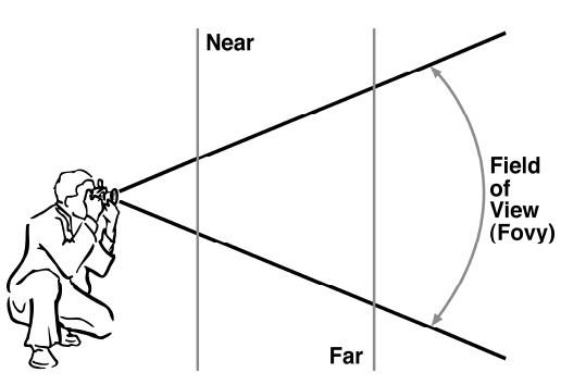
另外一种经常使用的方式是通过视角(Fov)，宽高比(Aspect)来指定透视投影，例如旧版中函数gluPerspective，参数形式为：

API void gluPerspective(GLdouble fovy, GLdouble aspect, GLdouble zNear, GLdouble zFar);

其中指定fovy指定视角，aspect指定宽高比，zNear和zFar指定剪裁平面。fovy的理解如下图所示(来自opengl 投影)：
fov

这些参数指定的是一个对称的视见体，如下图所示(图片来自Working with 3D Environment)：
perspective

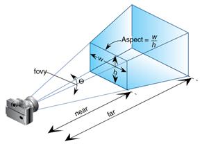
由这些参数，可以得到：
h=near∗tan(θ2) <script id="MathJax-Element-406" type="math/tex">h = near*tan(\frac{\theta}{2})</script>
w=h∗aspect <script id="MathJax-Element-407" type="math/tex">w=h*aspect</script>
对应上述透视投影矩阵中：
r=−l,r=w <script id="MathJax-Element-408" type="math/tex">r=-l,r=w</script>
t=−b,t=h <script id="MathJax-Element-409" type="math/tex">t=-b, t=h</script>
则得到透视投影矩阵为：

P = ⎡ ⎣ ⎢ ⎢ ⎢ ⎢ ⎢ ⎢ ⎢ ⎢ ⎢ ⎢ ⎢ c o t ( θ 2 ) a s p e c t 000 0 c o t (θ 2) 00 00 - ( f + n ) f - n - 1 00 - 2 f n f - n 0 ⎤ ⎦ ⎥ ⎥ ⎥ ⎥ ⎥ ⎥ ⎥ ⎥ ⎥ ⎥ ⎥ (Fov 透 视 投 影 矩 阵)

正交投影矩阵的推导

相比于透视投影，正交投影矩阵的推导要简单些，如下图所示：

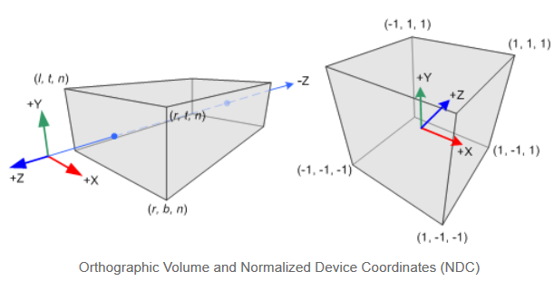
对于正交投影，有 xp=xe,yp=ye <script id="MathJax-Element-3131" type="math/tex">x_{p}=x_{e},y_{p}=y_{e}</script>，因而可以直接利用 xe <script id="MathJax-Element-3132" type="math/tex">x_{e}</script>与 xn <script id="MathJax-Element-3133" type="math/tex">x_{n}</script>的映射关系： [l,−1],[r,1] <script id="MathJax-Element-3134" type="math/tex">[l,-1],[r,1]</script>，利用 ye <script id="MathJax-Element-3135" type="math/tex">y_{e}</script>和 yn <script id="MathJax-Element-3136" type="math/tex">y_{n}</script>的映射关系： [b,−1],[t,1] <script id="MathJax-Element-3137" type="math/tex">[b,-1],[t,1]</script>，以及 ze <script id="MathJax-Element-3138" type="math/tex">z_{e}</script>和 zn <script id="MathJax-Element-3139" type="math/tex">z_{n}</script>的映射关系： [−n,−1],[−f,1] <script id="MathJax-Element-3140" type="math/tex">[-n,-1],[-f,1]</script>。例如 xe <script id="MathJax-Element-3141" type="math/tex">x_{e}</script>与 xn <script id="MathJax-Element-3142" type="math/tex">x_{n}</script>的映射关系表示为如下图所示：

x分量的映射关系

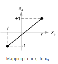
利用 [l,−1],[r,1] <script id="MathJax-Element-3143" type="math/tex">[l,-1],[r,1]</script>得到:

xn=2r−lxe−r+lr−l(2.1) <script id="MathJax-Element-3144" type="math/tex">x_{n} = \frac{2}{r - l}x_{e} - \frac{r + l}{r - l} \tag{2.1}</script>
同理可得到y,z分量的关系式为：
yn=2t−bye−t+bt−b(2.2) <script id="MathJax-Element-3145" type="math/tex">y_{n} = \frac{2}{t - b}y_{e} - \frac{t + b}{t - b} \tag{2.2}</script>
zn=−2f−nze−f+nf−n(2.3) <script id="MathJax-Element-3146" type="math/tex">z_{n} = \frac{-2}{f-n}z_{e}-\frac{f + n}{f - n} \tag{2.3}</script>

对于正交投影而言，w成分是不必要的，保持为1即可，则所求投影矩阵第四行为(0,0,0,1)，w保持为1，则NDC坐标和剪裁坐标相同，从而得到正交投影矩阵为:

O = ⎡ ⎣ ⎢ ⎢ ⎢ ⎢ ⎢ ⎢ ⎢ ⎢ ⎢ ⎢ 2 r - l 000 0 2 t - b 00 00 - 2 f - n 0 - r + l r - l - t + b t - b - f + n f - n 1 ⎤ ⎦ ⎥ ⎥ ⎥ ⎥ ⎥ ⎥ ⎥ ⎥ ⎥ ⎥ (正 交 投 影 矩 阵)

如果视见体是对称的，即满足 r=−l,t=−b <script id="MathJax-Element-3148" type="math/tex">r=-l,t=-b</script>，则矩阵O可以简化为：

O = ⎡ ⎣ ⎢ ⎢ ⎢ ⎢ ⎢ ⎢ ⎢ ⎢ ⎢ 1 r 000 0 1 t 00 00 - 2 f - n 0 00 - f + n f - n 1 ⎤ ⎦ ⎥ ⎥ ⎥ ⎥ ⎥ ⎥ ⎥ ⎥ ⎥ (简 化 正 交 投 影 矩 阵)

利用平移和旋转推导正交投影矩阵

还可以看做把视见体的中心移动到规范视见体的中心即原点处，然后缩放视见体使得它的每条边长度都为2，进行这一过程的变换表示为：

O = S (2 / (r - l), 2 / (t - b), 2 / (n e a r - f a r)) * T (- (r + l) / 2, - (t + b) / 2, (f + n) / 2) = ⎡ ⎣ ⎢ ⎢ ⎢ ⎢ ⎢ ⎢ ⎢ ⎢ ⎢ 2 r - l 000 0 2 t - b 00 00 2 n - f 0 0001 ⎤ ⎦ ⎥ ⎥ ⎥ ⎥ ⎥ ⎥ ⎥ ⎥ ⎥ * ⎡ ⎣ ⎢ ⎢ ⎢ ⎢ ⎢ ⎢ ⎢ ⎢ ⎢ 100001000010 - r + l 2 - t + b 2 f + n 2 1 ⎤ ⎦ ⎥ ⎥ ⎥ ⎥ ⎥ ⎥ ⎥ ⎥ ⎥ = ⎡ ⎣ ⎢ ⎢ ⎢ ⎢ ⎢ ⎢ ⎢ ⎢ ⎢ ⎢ 2 r - l 000 0 2 t - b 00 00 - 2 f - n 0 - r + l r - l - t + b t - b - f + n f - n 1 ⎤ ⎦ ⎥ ⎥ ⎥ ⎥ ⎥ ⎥ ⎥ ⎥ ⎥ ⎥

视口变换矩阵的推导

视变换是将NDC坐标转换为显示屏幕坐标的过程，如下图所示：

视口变换
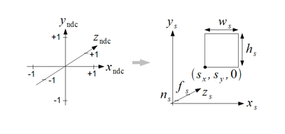
视口变化通过函数:
glViewport(GLint sx <script id="MathJax-Element-3235" type="math/tex">s_{x}</script> , GLint sy <script id="MathJax-Element-3236" type="math/tex">s_{y}</script> , GLsizei ws <script id="MathJax-Element-3237" type="math/tex">w_{s}</script> , GLsizei hs <script id="MathJax-Element-3238" type="math/tex">h_{s}</script>);
glDepthRangef(GLclampf ns <script id="MathJax-Element-3239" type="math/tex">n_{s}</script> , GLclampf fs <script id="MathJax-Element-3240" type="math/tex">f_{s}</script> );

两个函数来指定。其中( sx <script id="MathJax-Element-3241" type="math/tex">s_{x}</script>, sy <script id="MathJax-Element-3242" type="math/tex">s_{y}</script>)表示窗口的左下角， ns <script id="MathJax-Element-3243" type="math/tex">n_{s}</script>和 fs <script id="MathJax-Element-3244" type="math/tex">f_{s}</script>指定远近剪裁平面到屏幕坐标的映射关系。
使用线性映射关系如下：

(−1,sx),(1,sx+ws)(x分量映射关系) <script id="MathJax-Element-3245" type="math/tex">(-1,s_{x}),(1,s_{x}+w_{s}) \tag{x分量映射关系}</script>
(−1,sy),(1,sy+hs)(y分量映射关系) <script id="MathJax-Element-3246" type="math/tex">(-1,s_{y}),(1,s_{y}+h_{s}) \tag{y分量映射关系}</script>
(−1,ns),(1,fs)(z分量映射关系) <script id="MathJax-Element-3247" type="math/tex">(-1,n_{s}),(1,f_{s}) \tag{z分量映射关系}</script>

求出线性映射函数为:
xs=ws2xn+sx+ws2(3.1) <script id="MathJax-Element-3248" type="math/tex">x_{s}=\frac{w_{s}}{2}x_{n}+s_{x}+\frac{w_{s}}{2} \tag{3.1}</script>
ys=hs2yn+sy+hs2(3.2) <script id="MathJax-Element-3249" type="math/tex">y_{s} = \frac{h_{s}}{2}y_{n}+s_{y}+\frac{h_{s}}{2} \tag{3.2}</script>
zs=fs−ns2zn+ns+fs2(3.3) <script id="MathJax-Element-3250" type="math/tex">z_{s}= \frac{f_{s}-n_{s}}{2}z_{n}+\frac{n_{s} + f_{s}}{2} \tag{3.3}</script>
则由上述式子得到视口变换矩阵为：

v i e w P o r t = ⎡ ⎣ ⎢ ⎢ ⎢ ⎢ ⎢ ⎢ ⎢ ⎢ ⎢ w s 2 000 0 h s 2 00 00 f s - n s 2 0 s x + w s 2 s y + h s 2 n s + f s 2 1 ⎤ ⎦ ⎥ ⎥ ⎥ ⎥ ⎥ ⎥ ⎥ ⎥ ⎥ (视 口 变 换 矩 阵)

Zfighting问题

回过头去看透视投影部分， zn <script id="MathJax-Element-4941" type="math/tex">z_{n}</script>与 ze <script id="MathJax-Element-4942" type="math/tex">z_{e}</script>的关系式1.10：
zn=−f+nf−nze−2fnf−n−ze(1.10) <script id="MathJax-Element-4943" type="math/tex">z_{n}=\frac{-\frac{f+n}{f-n}z_{e}-\frac{2fn}{f-n}}{-z_{e}}\tag{1.10}</script>
这是一个非线性关系函数，作图如下：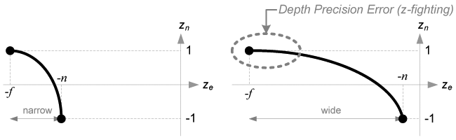
zfighting
从左边图我们可以看到，在近裁剪平面附近 zn <script id="MathJax-Element-4944" type="math/tex">z_{n}</script>值变化比较大，精确度较好；而在远裁剪平面附近，有一段距离内， zn <script id="MathJax-Element-4945" type="math/tex">z_{n}</script>近乎持平，精确度不好。当增大远近裁剪平面的范围 [−n,−f] <script id="MathJax-Element-4946" type="math/tex">[-n,-f]</script>后，如右边图所示，我们看到在远裁剪平面附近，不同相机坐标 ze <script id="MathJax-Element-4947" type="math/tex">z_{e}</script>对应的 zn <script id="MathJax-Element-4948" type="math/tex">z_{n}</script>相同，精确度低的现象更为明显，这种深度的精确度引起的问题称之为zFighting。要尽量减小[-n,-f]的范围，以减轻zFighting问题。